INTERACTING THROUGH DISCLOSING: PEER INTERACTION PATTERNS BASED ON SELF DISCLOSURE LEVELS VIA FACEBOOK

3467

LOSSLESS CODING SCHEME FOR DATA AUDIO 2

CHANNEL USING HUFFMAN AND SHANNON-FANO

1_{TONNY HIDAYAT,} 2_{MOHD HAFIZ ZAKARIA,} 3_{AHMAD NAIM CHE PEE}

1_{Universitas AMIKOM Yogyakarta, Department of Information Technology, Yogyakarta, Indonesia}

2,3_{Universiti Teknikal Malaysia Melaka, Faculty of Information and Communication Technology, Melaka,}

Malaysia

E-mail: 1_{tonny@amikom.ac.id,} 2_{hafiz@utem.edu.my,} 3_{naim@utem.edu.my}

ABSTRACT

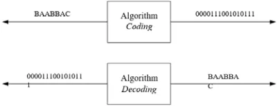
This paper shows the comparison of various lossless compression techniques. This research only concerns on audio the WAV 2 channel audio format. If an audio is said to be stereo, it means it has 2 channels (left channel and right channel). The code prefix to be generated becomes more and may appear more diverse. In this paper gives little change in the rule model for the allocation of bits to the prefix code generated. It gives different conclusions on the size and time ratios, toward existing research. The result of compression can accelerate transmission of information from one individual to another. Compression requires a technique which can be strategy against the pack of data. Information that can be compressed not only text but it can be Audio, pictures and video information. Furthermore, lossless compression is the most approach which is frequently used in data compression. Lossless compressions consist of some algorithm, such as Huffman, Shannon-Fano, Lempel Ziv Welch and run-length encoding. Each algorithm can play out another pressure. Finally, this paper generates the conclusion about the comparison of performance in Huffman and Shannon-Fano based on discussion of the result. The conclusions are difference result of compression-decompression speed and compression factor and ratio both of this algorithm.

Keywords: Audio, Lossless, WAV, Compression, Huffman, Shannon-fano

1. INTRODUCTION

The communication system is designed to transmit information that is generated by a source of multiple destinations. Source of information has a number of different forms. For example, in radio broadcasting, the source is usually in form of audio (voice or music). In TV broadcasting, information sources is usually a video that outputs in the form of the moving image. The output from these sources is an analog signal, and the source is called an analog source. Otherwise, computer and data storage such as magnetic or optical disks, generate output in the form of discrete signal (usually binary or ASCII characters) and the source is called a discrete source [1].

The lossless data compression consists of a conversion of data input to output data of which size is smaller because it uses reduction of data redundancy [2]. It can be achieved by assigning shorter code word to more frequent symbols in input data (a statistical compression) or by replacing possibly longest substrings with their dictionary codes (a dictionary compression). There are compression methods which use one or both of these

approaches. In the paper, we focus on details of approaches as sources of ideas for our method[3].

Figure 1. Lossless Compression Illustration

The source stemming analog or discrete, digital communications is designed to transmit information in digital form. Consequently, the output of the source must be changed previously into digital source output which is usually done on the source encoder, the output can be assumed to be a binary digit sequential [1].

3468 The first model appears for the digital signal compression. The model is the Shannon-Fano Coding. Shannon and Fano (1948) develop this algorithm which generates the binary code word for each symbol in the data file[1].

Huffman coding [1952] uses almost of all the characteristics of the Shannon-Fano coding. Huffman coding can produce an effective data compression by reducing the amount of redundancy in the coding symbol. It has been proven, that the Huffman Coding occurring fixed-length method is the most efficient[1][4].

In fifteen years, Huffman Coding has been replaced by arithmetic coding. Arithmetic coding attempt to replace a symbol input with a specific code. This algorithm replaces a stream of symbols input with a numeric floating-point single output. More bits are needed in the output numbers, and it causes the more complicated of received message[4]. Dictionary-based compression algorithm uses a very different method for compressing the data. This algorithm replaces the variable-length string of symbols into a token. The token is an index in the order of words in the dictionary. When the token is smaller than the word, so the token will replace the phrase and compression occurs. There are many methods and compression algorithms, but in this paper will be discussed the method of compression using Huffman, Shannon-Fano and Adaptive Huffman[1][4][3].

The important thing in data compression is the removal of redundancy. After redundancy is omitted, the information must be encoded into binary code. In the implementation phase, shorter code words are used to represent letters that appear more frequently in order to reduce the number of bits needed to represent each letter.

The same situation exists in digital communication. The speed in the communication channel, either through cable or wireless, is increasing slowly. Therefore the data sent between telephone lines, fax machines, mobile phones, even a set can be compressed. The data uploaded to an internet site is also compressed when uploaded or downloaded.

In this study, statistical analysis and performance comparison of the Shannon-Fano and Huffman algorithms were performed on WAV 2 Channel Audio file compression. Judging from the speed of the compression and decompression process, the required memory ratio or the size of the

compressed file to the original file) and the proof that no data is lost or changed.

The expected advantage of this research is to determine the optimal algorithm in the compression process of WAV 2 Channel audio data so as to minimize memory or bandwidth usage, speed up the data transmission process.

2. THEORY

In Lossless compression, the information contained in the result file is the same as the information in the original file. The resulting file compression process can be perfectly restored to the original file, no loss of information, no information error. Therefore, this method is also called error-free compression. Because it must maintain the perfection of information, so there is only the process of coding and decoding, there is no process of quantitation. This type of compression is suitable to apply to database files, spreadsheets, word processing files, biomedical images and audio.

The basic view of source coding is to remove redundancy from the source. Source Coding produces data and reduces the rate of compression transmission. Reduction of the rate of transmission can reduce the cost of connection and gives the user the possibility to share the same connection. In general, we can to compress data without removing information (lossless source coding) or compressing data with the loss of information (the loss of source coding) [5].

The theory of Source Encoding is one of the three fundamental theorems of information theory introduced by Shannon (1948). The theory of Source Encoding declared a fundamental limit of a size where the output of sources of information can be compressed without causing a huge error probability. We already know that the entropy of a source of information is a measure of the information content of a resource. So, from opinion the theory source encoding that the entropy of a source is very important[1][4][6].

The source is determined by the efficiency of H (X)/H (X) max, where pi is the probability of symbol to-I, and H (X) maximum when sources have the same probability of symbol [7][8][9][10].

3469 Where Pi is a probability of occurrence of an i-th symbol of the alphabet. Redundancy is a difference between the maximum theoretical entropy of the data and it has actual entropy. It is calculated as follow:

where P represents the highest entropy symbol ratio (P = 1/n).

Shannon's Noiseless Source Coding theory states that the average value of binary symbols per output source can be used to reach the entropy of the source. In other words, the efficiency of the resources can be generated from source coding. For the resource with the same symbol, the probability and statistics are not tied to the other, and then it can be encode each symbol in a code word of length n[11].

In this paper is discussed and analyzed source encoding based on a mathematical model of resource information and quantitative measurement of the information which is generated by the source.

Figure 2. The Classification Of Lossless Compression Techniques[12] [13][14][15].

2.1 A Statistical Approach

Consequences of factual perceptions can be fused into information compression techniques. The insights might be gotten by breaking down information (frequencies of symbols or words) or be given from the earlier from more broad perceptions (i.e., letter, di-and trigrams frequency in a language). The thought behind this approach is to utilize a variable estimated prefix code and appoint briefest code words to the most successive substrings in the source or to utilize an entropy encoding in light of scopes of numbers with go width relative to substring probabilities[3].

A prefix code, by and large, is a variable estimated code where none of the codewords can be

a prefix of the other. The codewords are created on a paired tree. The symbols are leaves and a course to leaves is coded by bits (1 for the left youngster and 0 for the privilege on each level of the tree). Leaves with the most successive symbols are nearer to the base of the tree and in this manner have shorter codes. This code is normally created by both - a coder and a decoder. The coder tallies events of every image and spares acquired esteems into the yield, so the decoder can manufacture a similar code tree. The decoder just peruses input bit-by-bit and goes down the tree picking the correct kid each time it peruses 0 and the left kid when it peruses 1. At the point when decoder achieves a leaf it peruses an encoded image and begins again from the root. There is additionally a versatile variation of Huffman coding, where a tree is remake powerfully when handling consequent info symbols (more often than not it is a superior answer for on-line compression, when input information can't be prepared twice).

Unary coding is the least complex coding strategy where codeword is made by n "set bits" trailed by one "reset bit" (i.e. 111110 speaks to esteem 5). A general unary code is made of two sections: an unary advance number and n-bits paired esteem. The codewords are produced by the begin step-stop calculation. The resulting parameters have the accompanying importance: begin is equivalent to the underlying length of a paired part, step decides addition of the parallel part and stop decides the longest codeword estimate (on account of the longest codewords, the progression number isn't trailed by the reset bit). For the situation when the progression is equivalent to 1, this code is very like Elias Gamma code that is built of l-zeros took after by one and a parallel piece of length l.

2.2 Algorithm of Huffman Coding

In the Huffman Coding, a long block from the source output is mapped to the binary blocks based on post variable. This way is referred to as fixed to variable-length coding. The basic idea of how this is starting to map a Huffman symbol most widely found in a source sequence to the binary sequence appear to be jarring. In the variable-length coding, synchronization is a problem. This means there must be a way to break the binary sequence is received into a code word[16] [17].

3470 code word with a length of 1/pi and at the same time can ensure that can uniquely encode, We can find the average length of the code H (x). Huffman Code can be uniquely decoding has with H (x) minimum, and optimum on the uniqueness of the codes[18] [19] [5].

The algorithm of Huffman encoding is:

1. Sorting output source starts with the highest

probability[20].

2. Combine two outputs the same close into one

output probability is the sum of probabilities before[21][22].

3. If after the split there is still two outputs, then

continue to the next step, but if there are still more than 2, return to step 1[23].

4. Give it a value of 0 and 1 for the second

output[3].

5. If an output is a result of merging two output

from the previous step, then give the sign of 0 and 1 for the code word, repeat until the output is one output that stands on its own[24].

Figure 3. Huffman Code Program Flow[25]

2.3 Shannon-Fano Algorithm Encoding

Shannon-Fano coding technique is one of the first algorithms whose goal is creating a code word with minimum redundancy. The basic idea is creating a code word with variable-length code, such as Huffman codes, and discovered a few years later[26].

As mentioned above, Shannon-Fano coding based on variable length-word, has means that some of the symbols in the message (which will be encoded) is represented with a code word. It is shorter than the existing symbol in the message. The

higher the probability makes the code word is getting short [19][27].

Estimating the length of each code word can be determined from the probability of each symbol and it is represented by the code word. Shannon-Fano coding generates a code word that has not the same length, so the code is unique and can be encoded[28][29].

The efficient of other variable-length coding in Shannon-Fano can be done. So, it needs steps for encoding well. The procedure in the Shannon-Fano encoding are:

1. Compile a probability of a symbol of the source

of the highest to the lowest [30].

2. Divide into 2 equal parts, and provide a value 0

for the top and once for the bottom [21].

3. Repeat step 2, each Division with an equal

probability up to impossible to divide again [20].

4. Encodes each symbol of the original source

being a binary sequence generated by the Division of each process [20][12].

3. ANALYSIS AND COMPARISON

There are different criteria to measure the performance of a compression algorithm. However, the main concern has always been the space efficiency and time efficiency.

Compression Ratio is a ratio between the size of the compressed file and the size of the source file. The compression factor is the inverse of the compression ratio [31][32][33][34][35].

100

100

Speed (in compression and

3471

Comparing the results of a lossless compression especially on WAV audio data is very difficult to get assumptions which algorithm is better, because various researches with audio data objects do not have the same data, there are public and private. Research in the field of image processing using data and objects are always the same, making it easier for researchers in comparing and looking for novelty. In the study using audio data that is public, some previous research already exists that use this data for test data.

To conduct data compression program simulation in Matlab, we use WAVE Sound file (*.Wav). This file was originally (J.S.Bach; Partita E major, Gavotte en rondeau (excerpt) - Sirkka

Väisänen, violin), from resource

http://www.music.helsinki.fi/tmt/opetus/uusmedia/e sim/index-e.html.

The data file is “a2002011001-e02.wav” (Original recording (PCM encoded 16 bits per sample, sampling rate 44100 Hertz, stereo, Duration 54.3 Second ). Size 9.13 MB (9,580,594 bytes).

Problems will be analyzed, and processed are:

1. The influence of the number of symbols against

the gain compression.

2. The influence of the abundance frequencies of

each symbol against the gain compression.

3. The entropy value against the influence of gain

compression.

4. The advantages of each method of compression

used in the simulation program.

5. Lack of each compression method used in a

simulation program.

Algorithm for Huffman coding:

Huffman algorithm procedure based on research on the optimum prefix code is.

1. Symbols that have a frequency of appearances

more often will have a code word shorter than other symbols.

2. Two symbols that have the least number of

occurrences will have a code word of the same length

Data structure used: Priority queue = Q, A is given alphabet

Huffman (c) { n = |c| Q = c For i = 1 to n-1

{

do Z = Allocate-Node ()

x = left[z] = EXTRACT_MIN (Q) y = right[z] = EXTRACT_MIN (Q) F[z] = F[x] + F[y] INSERT (Q, z) } return EXTRACT_MIN (Q) }

Complexity is O (n log n), each priority queue of complexity is O (log n).

Limitations of Huffman Coding:

1. This code gives an optimal solution when

only if the exact probability distribution of the source symbols is known.

2. The encoding of each symbol is with an

integer number of bits.

3. When changing the source statistics then

Huffman coding is not efficient.

4. Due to the large length of the least probable

symbol of this code. So, storage in a single word or basic storage is complex.

A Shannon– Fano tree is worked by a particular intended to characterize a successful code table.

This method begins with a sequence of symbols with known frequency occurrence. Then the set of symbols is divided into two parts that weigh the same or almost the same. All symbols on subset are given binary 0, while the symbols on subset II are binary 1. Each subset is subdivided into two subsets with the same as subset I and subset II. If a subset contains only two symbols, a binary is assigned to each symbol The process will continue until no subset is left

1. For a given rundown of symbols, build up a

comparing rundown of probabilities or frequency checks with the goal that every symbol’s relative frequency of event is known.

2. Sort the arrangements of symbols as indicated by

frequency, with the most as often as possible happening symbols at the left and minimal regular at the privilege.

3. Divide the rundown into two sections, with the

aggregate frequency checks of the left part being as near the aggregate of the great.

4. The left piece of the rundown is allocated the

parallel digit 0, and the correct part is relegated the digit 1. This implies the codes for the symbols in the initial segment will all begin with 0, and the codes in the second part will all begin with 1.

5. Recursively apply the step 3 and 4 to every one

3472 every image has turned into a relating code leaf on the tree.

comp_t = 0;

for i = 1 : size(signal,2)

[us,~,ic] = unique(signal(:,i)); us2{1,i} = us;

p = tabulate(signal(:,i)); p(p(:,2) == 0,:) = []; p = p(:,2);

p = reshape(p,1,length(p)); p2{1,i} = p;

tic;

codex = norm2sf(p); codexx{1,i} = codex; codex2 = codex(ic);

info = cellfun('length',codex2); info2{1,i} = info;

signal_comp{1,i} = cell2mat(codex2'); comp_t = toc+comp_t;

end

dcomp_t = 0;

for i = 1 : size(signal,2) tic;

dsig2 =

sf2norm(signal_comp{1,i},codexx{1,i},us2{1,i},inf o2{1,i});

dsig(:,i) = dsig2'; dcomp_t = toc+dcomp_t; end

The Entropy of the source.

H

The average length of the Shannon-Fano code is

Lavg

Thus the efficiency of the Shannon-Fano code is

H Lavg

Following is the result of compression:

Figure 4. waveform graph the results of Huffman and Shannon-fano with File Original

The result of decompression can be seen from waveform figure 4, that there is no change or reduction of data according to the principle of lossless compression.

The results of testing these two methods are as follows :

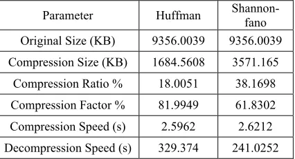
Table 1. Result Compression Huffman and Shannon-fano

Parameter Huffman Shannon-_fano

Original Size (KB) 9356.0039 9356.0039 Compression Size (KB) 1684.5608 3571.165

Compression Ratio % 18.0051 38.1698 Compression Factor % 81.9949 61.8302 Compression Speed (s) 2.5962 2.6212 Decompression Speed (s) 329.374 241.0252

Table 2. Result Coding Huffman and Shannon-fano

Shannon-fano Channel 1

Letter Prob Count Length Num of _Bit

0 2.92E-05 70 12 840

1 3.67E-05 88 12 1056

2 8.39E-05 201 11 2211

3 1.69E-04 405 10 4050

4 2.84E-04 680 10 6800

5 5.21E-04 1247 9 11223

6 9.03E-04 2162 9 19458

7 0.0016 3787 8 30296

8 0.003 7197 7 50379

9 0.0056 13439 6 80634

10 0.0101 24078 6 144468

11 0.0187 44757 5 223785

12 0.0338 80883 4 323532

(3)

3473

13 0.0639 152959 4 611836

14 0.1221 292556 3 877668

15 0.2387 571657 3 1714971

16 0.242 579615 2 1159230

17 0.122 292302 3 876906

18 0.0626 149948 4 599792

19 0.033 79120 5 395600

20 0.0178 42679 5 213395

21 0.0098 23451 6 140706

22 0.0056 13402 7 93814

23 0.0033 8016 7 56112

24 0.002 4886 8 39088

25 0.0011 2661 8 21288

26 5.75E-04 1376 9 12384

27 3.02E-04 723 10 7230

28 1.54E-04 368 10 3680

29 8.89E-05 213 11 2343

30 3.26E-05 78 12 936

31 5.55E-05 133 12 1596

Shannon-fano Channel 2

Letter Prob Count Length Num of _Bit

4 1.42E-05 34 14 476

5 6.26E-05 150 12 1800

6 2.10E-04 502 12 6024

7 5.81E-04 1392 10 13920

8 0.0015 3547 9 31923

9 0.0031 7383 8 59064

10 0.0065 15508 7 108556

11 0.0133 31742 6 190452

12 0.0278 66631 5 333155

13 0.0574 137586 4 550344

14 0.1204 288364 3 865092

15 0.2699 646554 2 1293108

16 0.2673 640235 2 1280470

17 0.1223 292844 3 878532

18 0.0574 137364 4 549456

19 0.0272 65132 5 325660

20 0.013 31119 6 186714

21 0.0066 15733 7 110131

22 0.0032 7561 8 60488

23 0.0015 3474 9 31266

24 6.12E-04 1467 10 14670

25 2.19E-04 524 10 5240

26 8.23E-05 197 12 2364

27 2.92E-05 70 13 910

28 5.85E-06 14 15 210

29 3.76E-06 9 16 144

30 4.18E-07 1 16 16

Huffman Channel 1

Letter Prob Count Length Num of _Bit

0 2.92E-05 70 16 1120

1 3.67E-05 88 16 1408

2 8.39E-05 201 15 3015

3 1.69E-04 405 14 5670

4 2.84E-04 680 13 8840

5 5.21E-04 1247 12 14964

6 9.03E-04 2162 11 23782

7 0.0016 3787 10 37870

8 0.003 7197 9 64773

9 0.0056 13439 8 107512

10 0.0101 24078 7 168546

11 0.0187 44757 6 268542

12 0.0338 80883 5 404415

13 0.0639 152959 4 611836

14 0.1221 292556 3 877668

15 0.2387 571657 2 1143314

16 0.242 579615 2 1159230

17 0.122 292302 3 876906

18 0.0626 149948 4 599792

19 0.033 79120 5 395600

20 0.0178 42679 6 256074

21 0.0098 23451 7 164157

22 0.0056 13402 8 107216

23 0.0033 8016 9 72144

24 0.002 4886 10 48860

25 0.0011 2661 11 29271

26 5.75E-04 1376 12 16512

27 3.02E-04 723 13 9399

28 1.54E-04 368 14 5152

29 8.89E-05 213 15 3195

30 3.26E-05 78 16 1248

31 5.55E-05 133 16 2128

Huffman Channel 2

Letter Prob Count Length Num of _Bit

4 1.42E-05 34 15 510

5 6.26E-05 150 13 1950

6 2.10E-04 502 11 5522

7 5.81E-04 1392 10 13920

8 0.0015 3547 9 31923

9 0.0031 7383 8 59064

10 0.0065 15508 7 108556

11 0.0133 31742 6 190452

12 0.0278 66631 5 333155

13 0.0574 137586 4 550344

14 0.1204 288364 3 865092

3474

16 0.2673 640235 2 1280470

17 0.1223 292844 3 878532

18 0.0574 137364 4 549456

19 0.0272 65132 5 325660

20 0.013 31119 6 186714

21 0.0066 15733 7 110131

22 0.0032 7561 8 60488

23 0.0015 3474 9 31266

24 6.12E-04 1467 10 14670

25 2.19E-04 524 10 5240

26 8.23E-05 197 12 2364

27 2.92E-05 70 14 980

28 5.85E-06 14 16 224

29 3.76E-06 9 17 153

30 4.18E-07 1 17 17

From the calculation of memory capacity used after the decoding process is done, it looks different that may not look big. However, when it is an audio data that many variations of waveform, then the number of memory capacity is very instrumental in determining the more effective compression. This is more because the Huffman algorithm can form a more efficient prefix form than Shannon-fano. Compared with ASCII code means Huffman algorithm uses only 30% bit only. Since one character has 8 bits in the ASCII code, it means that at 100 times there are 800 bits. In other words, Huffman can compress files up to 80% and Shannon-fano can only file 60% based on above test. This result cannot be beaten flat for all files, but this as an illustration for comparison only. The Shannon-fano algorithm works in conjunction with the Huffman algorithm in a particular case (depending on the probability of character occurrence).

The results of compression in Table 1 and Table 2 give different results from several existing studies as follows :

1. In the compression survey Table 3. between

RLE, LZW and Huffman, in this paper the result is Huffman Fast to Execute [37].

Table 3. Compression between of the Lossless Compression algorithm[37]

2. Considering the size, there is a further reduction

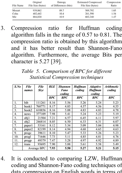
in the file size. The compressed file sizes are about 60% of the original files. Further reductions can be obtained by using more sophisticated models. Many of the lossless audio compression schemes, including FLAC (Free Lossless Audio Codec), Apple's ALAC or ALE, Shorten, Monkey's Audio, and the MPEG-4 ALS algorithms, use a linear predictive model to remove some of the structure from the audio sequence and use Rice coding to encode the residuals. Most others, such as AudioPak and OggSquish, use Huffman coding to encode the residuals[38].

Table 4. Huffman coding of differences of 16-bit CD-quality audio

3. Compression ratio for Huffman coding

algorithm falls in the range of 0.57 to 0.81. The compression ratio is obtained by this algorithm and it has better result than Shannon-Fano algorithm. Furthermore, the average Bits per character is 5.27 [39].

Table 5. Comparison of BPC for different Statistical Compression techniques

4. It is conducted to comparing LZW, Huffman

3475 compression size, compression ratio, and saving percentage. After testing those algorithms, Huffman and ShannonFano coding are very

powerful than LZW. Huffman and

ShannonFano coding gives better results and can reduce the size [40].

Table 6. Comparison between LZW, Huffman Coding and Shannon-Fano coding

5. Comparison of Arithmetic and Huffman have

given in Table 2. Arithmetic coding of CR is higher than Huffman coding. Huffman coding takes less memory space than Arithmetic coding. Compression and decompression time of Huffman coding is slower than the Arithmetic coding[41][15].

Table 7. Comparison of Arithmetic & Huffman coding

6. If there are not miss the data then the

compression is called lossless compression. The Huffman coding comes with lossless compression. The obtained results shows that the input with the similar probability gives better compression ratio, space savings and average bits than the input with the different probability. The Huffman code gives better compression ratio, space savings and average bits as compared with the uncompressed data [27].

4. CONCLUSION AND FUTURE WORK

The testing results using Matlab, there is a big difference from the final result in Table 1. Huffman and Shannon-Fano can be concluded that

the result of lossless compression for the data WAVE Sound file (* .Wav) as follows:

1. Huffman decompression speed is slower than

Shannon-fano, while decompression rate is relatively same.

2. Shannon-fano compression gives the

compression ratio of 38.14% and compression factor is 61.85%, Huffman are 18.0051% and 81.9949%. Huffman is better than Shannon-Fano in compression ratio and factor.

3. A large number frequency of symbols and each

symbol determines the value of entropy a data. The entropy value is used to determine the gain compression.

4. If it has much more entropy value then there is

few obtained gain value at the time of compressing data.

The continuation of this research is trying to compare all of the lossless compression algorithms using the same data. So, it can give a better results of all the lossless compression methods.

5. ACKNOWLEDGED

This paper is an ongoing research on deeper lossless compression technique for music files. Thank you Universitas AMIKOM Yogyakarta and Universiti Teknikal Malaysia Melaka, and everyone who provided substantial support in this study.

REFERENCES:

[1] S. Mishra, “A Survey Paper on Different Data Compression Techniques Saumya Mishra shraddha singh,” no. May, pp. 738–740, 2016. [2] C. E. Shannon, “A mathematical theory of

communication,” Bell Syst. Tech. J., vol. 27,

no. July 1928, pp. 379–423, 1948.

[3] M. Ch??opkowski and R. Walkowiak, “A general purpose lossless data compression

method for GPU,” J. Parallel Distrib.

Comput., vol. 75, pp. 40–52, 2015.

[4] R. Kaur, “3 . Lossless Compression Methods : -,” vol. 2, no. 2, 2013.

[5] R. A. Bedruz and A. R. F. Quiros, “Comparison of Huffman Algorithm and Lempel-Ziv Algorithm for audio, image and

text compression,” 8th Int. Conf. Humanoid,

Nanotechnology, Inf. Technol. Commun.

Control. Environ. Manag. HNICEM 2015, no.

December, 2016.

[6] K. Sayood, Arithmetic Coding. 2012.

[7] G. Ulacha and R. Stasinski, “Lossless audio

coding by predictor blending,” 2013 36th Int.

Conf. Telecommun. Signal Process. TSP 2013,

3476 [8] G. Ulacha and R. Stasinski, “Novel ideas for

lossless audio coding,” 2012 Int. Conf. Signals

Electron. Syst. ICSES 2012 - Conf. Proc., no.

3, pp. 3–6, 2012.

[9] I. Conference and O. N. Electronics, “to Assess the Quality of Audio Codecs,” no. Icecs, pp. 252–258, 2015.

[10] K. Sayood, “Huffman Coding,” Introd. to Data

Compression, pp. 43–89, 2012.

[11] K. Khaldi, A. O. Boudraa, B. Torrésani, T. Chonavel, and M. Turki, “Audio encoding

using Huang and Hilbert transforms,” Final

Progr. Abstr. B. - 4th Int. Symp. Commun.

Control. Signal Process. ISCCSP 2010, no.

March, pp. 3–5, 2010.

[12] R. S. Brar, “A Survey on Different Compression Techniques and Bit Reduction Algorithm for Compression of Text / Lossless Data,” vol. 3, no. 3, pp. 579–582, 2013. [13] K. . Ramya and M. Pushpa, “A Survey on

Lossless and Lossy Data Compression

Methods,” Int. J. Comput. Sci. Eng. Commun.,

vol. 4, no. 1, pp. 1277–1280, 2016.

[14] A. Patil and R. Goudar, “A Survey of Different Lossless Compression Algorithms .,” vol. 1, no. 12, pp. 202–209, 2014.

[15] A. J. Maan, “Analysis and Comparison of Algorithms for Lossless Data Compression,”

Int. J. Inf. Comput. Technol., vol. Vol. 3, no.

No. 3, pp. 139–146, 2013.

[16] “13. Compression and Decompression.” [17] S. Karlsson, J. Marcus, and D. Flemstr,

“Lossless Message Compression Bachelor Thesis in Computer Science,” 2013.

[18] I. Pu et al., “Introduction to Data

Compression,” Sci. Eng. Guid. to Digit. Signal

Process., vol. 709, no. 4, p. xx + 636, 2013.

[19] S. Kumar, S. S. Bhadauria, and R. Gupta, “A Temporal Database Compression with

Differential Method,” Int. J. Comput. Appl.,

vol. 48, no. 6, pp. 65–68, 2012.

[20] B. Singh, “A Review of ECG Data Compression Techniques,” vol. 116, no. 11, pp. 39–44, 2015.

[21] D. Okkalides and S. Efremides, “International Conference on Recent Trends in Physics 2016

(ICRTP2016),” J. Phys. Conf. Ser., vol. 755, p.

11001, 2016.

[22] M. S. H. Ayyash, “IMPLEMENTATION OF A DIGITAL COMMUNUCATION SYSTEM IMPLEMENTATION OF A DIGITAL,” 2011.

[23] G. Brzuchalski and G. Pastuszak, “Energy balance in advanced audio coding encoder bit-distortion loop algorithm,” vol. 8903, p.

89031T, 2013.

[24] K. M. Fisher and K. Fisher, “Towards Understanding the Compression of Sound Information Towards Understanding the Compression of Sound Information,” 2016. [25] G. Gupta and P. Thakur, “Image Compression

Using Lossless Compression Techniques,” no. December, pp. 3896–3900, 2014.

[26] M. Vaidya, E. S. Walia, and A. Gupta, “Data compression using Shannon-fano algorithm

implemented by VHDL,” 2014 Int. Conf. Adv.

Eng. Technol. Res. ICAETR 2014, pp. 0–4,

2014.

[27] P. Ezhilarasu, N. Krishnaraj, and V. S. Babu, “Huffman Coding for Lossless Data Compression-A Review Department on

Information Technology , Valliammai

Engineering College ,” vol. 23, no. 8, pp. 1598–1603, 2015.

[28] K. Khaldi, A. O. Boudraa, B. Torresani, and M. Turki, “Audio encoding using Huang and Hilbert transforms,” no. March, pp. 3–5, 2010. [29] A. Aswin, A. G. Nair, N. Radhakrishnan, D. Kirandeep, and R. Gandhiraj, “Android Application using Qt for Shannon-Fano- Elias Decoding,” pp. 389–391, 2016.

[30] A. Zribi, R. Pyndiah, S. Zaibi, F. Guilloud, and

A. Bouallègue, “Low-complexity soft

decoding of huffman codes and iterative joint

source Channel Decoding,” IEEE Trans.

Commun., vol. 60, no. 6, pp. 1669–1679, 2012.

[31] R. A. Bedruz and A. R. F. Quiros, Comparison

of Huffman Algorithm and Lempel-Ziv Algorithm for audio, image and text

compression, no. December. 2016.

[32] P. V. Krishna, M. R. Babu, and E. Ariwa,

Global Trends in Computing and

Communication Systems, vol. 269. 2012.

[33] R. D. Masram and J. Abraham, “Efficient

Selection of Compression-Encryption

Algorithms for Securing Data Based on Various Parameters,” pp. 1–54, 2014.

[34] S. Porwal, Y. Chaudhary, J. Joshi, and M. Jain, “Data Compression Methodologies for Lossless Data and Comparison between Algorithms,” vol. 2, no. 2, pp. 142–147, 2014. [35] Y.-C. Hu and C.-C. Chang, “A new lossless compression scheme based on Huffman coding

scheme for image compression,” Signal

Process. Image Commun., vol. 16, no. 4, pp.

367–372, 2000.

[36] A. Odat, M. Otair, and M. Al-Khalayleh,

“Comparative study between LM-DH

technique and Huffman coding technique,” Int.

3477 36011, 2015.

[37] P. Kavitha, “A Survey on Lossless and Lossy Data Compression Methods,” vol. 7, no. 3, pp. 110–114, 2016.

[38] K. Sayood, Huffman Coding. 2012.

[39] S. Shanmugasundaram, “A comparative study

of text compression algorithms,” Int. J., vol. 1,

no. December, pp. 68–76, 2011.

[40] K. A. Ramya, M. Pushpa, and M. P. Student, “Comparative Study on Different Lossless Data Compression Methods,” no. 1, 2016. [41] G. Kumar, E. Sukhreet, S. Brar, R. Kumar, and