Information Technology and Economic Performance: A Global Analysis

Munich Personal RePEc Archive

Information Technology and Economic

Performance: A Global Analysis

Surfield, Christopher J.

Saginaw Valley State University

March 2008

Information Technology and Economic Performance: A Global Analysis

Christopher J. Surfield Saginaw Valley State University

Draft March 2009

ABSTRACT

INTRODUCTION

Information technologies such as the Internet or the personal computer are being embraced globally. These innovations are largely being viewed positive developments. Communications and knowledge can be quickly and easily transmitted across borders and across large distances. It is hoped that these

technologies can increase the productivity of an economy’s labor stock and, by extension, its growth. Perhaps with an eye towards obtaining these benefits, leaders of developing economies have begun to focus on creating and maintaining their technological infrastructures. As the costs of these technologies fall, this may be one cost-effective means that the developing world could exploit to increase their overall capital stocks.

However, within industrialized economies a different outlook on technology is being taken. Politicians fret that technology facilitates the movement of not just data and information across borders, but also jobs and employment. Unlike manufacturing and the production of goods, service-sector production was largely immune to the siren call of the plentiful cheap labor that can be found in

developing economies. The advent of the Internet, however, has freed companies from their geographic constraints when searching for qualified workers and new product markets. Labor, human capital, and customers can now be obtained from a broader market by a firm without actually relocating or adding new service centers. From the viewpoint of leaders in industrialized economies, no longer is it just the manufacturing jobs that are at risk for relocation to economies with lower labor costs, but now high-paying service jobs can be lost to low-wage economies.

on-line courses. In a related vein, if the increased use of technology improves labor productivity, additional output can be made available for global consumption.

The aim of this study is to statistically evaluate what ability, if any, that information technology has to increase economic growth. We extend the scope of our analysis to also provide estimates on any differentials that are attached to the use of these technologies by industrialized economies. We examine three distinct measures of economic performance. Namely, we take the amount of output produced per worker, the real per capita Gross Domestic Product (GDP), and the employment-population ratio as proxies for an economy’s performance. To facilitate this study, we analyze three international sources of data. All three datasets cover member states of the United Nations (UN), giving us a large pool of observations. Both cross section and panel data estimation techniques are adopted to provide estimates of the impact that information technology has on economic growth. We discuss the data and empirical strategies in sections 2 and 3, respectively. Our estimation results is contained in section 4, with concluding remarks presented in section 5.

DATA

As noted in our introduction, three different sources of data are exploited in this study. The first, which provides us with two out of our three dependent variables, is the Penn World Table, Version 6.1 (PWT 6.1). A commonly used dataset,1 the PWT 6.1 provides data that is both consistent in definition and in real terms across one hundred and sixty economies. It is a panel that spans the 1950 to 2000 time period, although we only analyze the 1993 – 2001 annual data. We extract from the PWT 6.1 both the per capita real GDP as well as the real GDP produced per worker. Both terms are expressed in dollar terms to facilitate comparisons across economies.

Our third measure of an economy’s performance is its Employment-Population Ratio (EPR). The EPR is calculated using data contained in the International Labour Office’s (ILO) Laborsta database.

1

Charged with the collection of labor market statistics across all UN member states,2 the ILO publishes estimates of the total number of employed workers. We then take these estimates and divide them by the total number of citizens residing in a member state. For ease in interpretation, we multiply the product by one hundred. The use of the EPR is preferable over an economy’s unemployment rate for several reasons. The first difficulty in using unemployment rates is the disparity in the definitions that each economy uses to measure unemployment. For example, the United States considers only those workers who are over the age of sixteen and actively seeking a job to be unemployed. Developing economies often include younger workers in the calculation of their rolls of unemployed workers. One such example, Brazil, counts those over the age of ten and seeking employment to be unemployed.

Differences in unemployment rates across developing and industrialized economies, therefore, may not be reflective of differences in technology stocks, but rather attributed to definitional issues. Second, there is a concern that the definition of unemployment is related to an economy’s ability to purchase technology, e.g. those economies who use a lower age in defining unemployment are also less likely to be able to afford technology. In these cases, we will obtain biased and inconsistent ordinary least squares results when regressing unemployment rates on technology stocks.

The use of the EPR sidesteps these concerns. Employed workers must satisfy only one condition; they must be employed. This definition is consistent across all economies and does not require that an age threshold be crossed before one is counted as being employed. This variable, however, will allow us to only indirectly draw inferences on the amount of joblessness that may be present within an economy. Higher EPRs can be interpreted as being the result of additional residents successfully acquiring offers of employment, but this may not necessarily mean that there are fewer unemployed workers. For example, it is possible that the numbers of unemployed workers remain constant in this case, with workers initially out of the labor force securing these offers of employment. The converse may also hold

2

if the EPR falls between two periods in time; the dislocated may opt to not search for employment and directly exit the labor force. While extreme examples, both situations are nonetheless possibilities and so changes in the EPR should be viewed with care.

Our two technology variables are both obtained from a publication that is provided by the International Telecommunications Union: the Yearbook of Statistics: Telecommunications Services 1992 – 2001 (to be hereafter referred to as the Yearbook). The Yearbook is the product of repeated annual questionnaires that are annually submitted to the statistical agencies within each UN member state that are responsible for the collection of telecommunications data. It is an ongoing survey first started in 1992. We do not use this initial round of data, however, due to the large number of incomplete observations. We instead begin our analysis with the 1993 data.

Our first measure of an economy’s information technology stock is the availability of personal computers (PerComp) for use within an economy. Taking into consideration the variation in economy populations, we standardize this measure. PerComp is calculated as the total number of computers available for each one hundred citizens ’ use. Although we cannot distinguish between the use of comp uters for productive from leisure purposes, we take PerComp as being our best proxy for an economy’s overall computer technology stock.

Our second technology variable is the annual aggregate investment made within each economy on its telecommunications infrastructure (TechInvest). Using both the consumer price indices and the average annual exchange rates that are published for each economy included in the Yearbook, we deflate the annual telecommunication investment amounts and convert them into (constant) dollar terms. Again, we standardize this variable to take into consideration the differing economy sizes; TechInvest is

reported as the number of dollars invested in telecommunications per citizen.

basis for distinguishing the developing economies from the industrialized economies. OECD is a dummy variable equal to one if economy i is a member of this organization at time t (zero otherwise). The interaction terms, OECD*PerComp and OECD*TechInvest, capture any differentials attaching to the use of computers and telecommunications investments, respectively, by industrialized countries. When using these two interaction terms, the initial technology variables provide estimates of any benefits that technology hold with respect to per capita real GDP, per worker real GDP, or the

employment-population ratio without regard to the level of industrialization. The interaction terms will adjust these estimates to reflect any advantage or disadvantage that OECD member states may ha ve in the incorporation of computers or investments in their production function.

Given that all three of our data sources span both a similar cross section of economies and time period, we can merge the technology and economic growth variables into four samples. We construct two cross section and two panel samples. The first cross section is used to provide inferences on the change in both the economic performance variables as well as technology variables from 1993 to 1997. The second cross examines the growth of an economy beginning in 1997 until 2000.

The justification for us ing the change in economic growth variables over a five year time period lies in when the data are collected. Many economies irregularly collect data on employment across years. For example, in 1993 the employed may be counted in February. The tabulations of the employed in a subsequent year, however, may be taken in January. If we were to use the changes in the EPR over a one year period, then it may be that the change from one year to the next may be attributed to

differences in when the employment survey is issued rather than being an actual change in employment levels. Over a longer time span, this measurement error, while still present, is minimized. Changes in the employment levels over five year intervals are more likely to reflect an actual change in the numbers of workers actually employed rather than seasonal or measurement issues.3

3

We face a significant concern in using the cross sections is that only those economies with comp lete data at both the initial and ending years can be included in the sample. In the first cross section, those economies for which we do not have economic and technology data in both 1993 and 1997 are excised from the sample, even if they report data for the interim years. Despite the best efforts of all three data sources, we confront the reality of a large number of missing values. This problem is particularly acute for our primary interest: developing economies.

Given this complication, we construct two panels that cover the same two time intervals as each cross section. The third and fourth samples used in this analysis cover the 1993 to 1997 and 1997 to 2000 time frame, respectively. We use panel data estimation techniques to not only provide more precise estimates of the impact that information technology has on economic growth, but also to control for economy-specific heterogeneity such as when the data are measured. In addition, those economies that have at least two annual observations within the time period covered by each panel are now eligible for inclusion in our multivariate analyses.

EMPIRICAL MODELS

As noted above, we have two distinct sample types. The cross sections examine the change in economic performance over a period of time. The pane ls, which express the data in annual levels, include the actual amounts of both the dependent and independent variables. Care must be taken in equating the results obtained from cross section results to those obtained from the panels. Both will provide similar inferences, although not necessarily in the same units or magnitudes. This section is partitioned into two; we first discuss our cross section model, then turn to the panel estimation strategy.

Changes in Economic Performance

Using the two cross sections and ordinary least squares (OLS), we estimate following model:

, ) (

) (

)

log( _{i,0 i,0 i,0 i i i}

i EPR PerComp TechInvest PerComp TechInvest

EPR =φ +α + β +δ ∆ +γ ∆ +ε

where∆EPR is the change in economy i’s employment-population ratio. The variables ∆PerComp and

TechInvest

∆ are the changes in economy i’s personal computer stocks and technology expenditures,

respectively, between year t and the initial year, 0. We include a normal idiosyncratic error term, ε. As noted in Durlauf, Johnson, and Temple (2004), an economy’s initial level of economic performance, e.g. the EPR of economy i at time 0, needs to be included in the regression model given the negative relationship found between rates of growth and their starting point. Put differently, we

expect φ to take on a negative sign. Intuitively, this implies that countries with a lower economic base

must grow quickly to catch up to their developed peers. The converse is that developed economies find it difficult to quickly increase their econo mic standing given their already large economic base. We take the natural log of the initial EPR to maintain consistency with the existing economic growth literature.

In the same vein, we also include the initial levels of technology (PerCompi,0and TechInvesti,0).

Again we would expect both α and β to be negatively-signed given that those economies with higher

stocks of technology experience lower growth rates if they maintain their steady-state growth paths. Our primary coefficients of interest, δ and γ , measure the impact that changes in the

availability of computers and technology investments have on econo mic growth, respectively. If, as hypothesized, these coefficients take on positive sign, it would imply that adding more computers with an economy or increased expenditures on technology translates into economic growth. In the model presented above, greater availability of computers or technology investment should increase the proportion of employed workers in an economy. Although the above discussion is focused on the evaluation of an economy’s employment-population ratio, the mechanics of the estimated models for both per capita real GDP and real GDP produced per worker operate in a similar manner.

Panel Data Estimation

we cannot include those economies for which we do not have data at both the beginning and ending years of each cross section. In light of these concerns, we turn to our two panel samples. One additional benefit realized from the use of these panels is the ability to use panel data estimation techniques, rather than the standard OLS, to provide more precise estimates of the implication that information technology holds for economic performance. To this end, we estimate both a random effect (RE) and fixed effect (FE) OLS model. Given that we have three distinct dependent variables, we shall again limit our discussion to the determination of an economy’s EPR. The models presented below can be generalized across the other two measures of economic growth.

Following Wooldridge (2001), the underlying employment-population rate determination model is as follows:

(

)

E i,t | i,t, i,t =δ i,t +γ i,t, =1,2,K (2)

where EPRi,tis the log of the annual employment-population ratio of economy i at time t. By using the

log of the dependent variable, we are effectively estimating an elasticity and the coefficient estimates for the two independent variables represent the percentage change in an economy’s EPR as it changes its technology stocks. This allows us at least a degree of comparability with the results obtained in the cross section. PerComp and TechInvest are not change variable as was the case earlier. Rather they are

expressed in level terms. PerComp is strictly speaking the total number of computers available for each one hundred citizens to use, with TechInvest being again the dollars spent per citizen on technology.

The parameters δ and γ are statistical estimates of the roles that PerComp and TechInvest play

in the determination of an economy’s EPR. Given equation (2), the estimated linear random effect model is therefore

T t

u TechInvest PerComp

EPR_{it it it it. 1,2,}K

, , ,

, =δ +γ + = (3)

The RE OLS model will provide us with unbiased and consistent estimates of both δ and γso

random effect OLS model will produce biased and inconsistent estimates of both δ and γ. That is to

say, in the presence of unobserved heterogeneity, the underlying unemployment rate determination model is not equation (2), but rather

T t c TechInvest PerComp TechInvest PerComp EPR

E( i,t | i,t, i,t)=δ i,t +γ i,t + i, =1,2,K (4)

with c_i being an economy-specific component influencing that economy’s EPR. The literature has

provided a number of examples in which economy-specific characteristics have a significant influence in the level of unemployment or economic growth enjoyed by a given economy.4 Given that we fail to observe such characteristics in our data, the RE OLS model estimates the following

T t

v TechInvest PerComp

EPRi,t =δ i,t +γ i,t + i,t, =1,2,K (5)

where vi,t =

(

)

(

)

therefore adopt the fixed effect linear model as our preferred panel data estimation technique. The FE OLS estimates T t u TechInvest PerComp

EPRi,t =αt +λi +δ i,t +γ i,t + i,t. =1,2,K (6)

In equation (6), αt is the year-specific intercept which captures any impact that time t has on all

employment-population ratios, with λ_i serving as an economy-specific intercept which controls for any

unobserved within-economy time- invariant characteristics.

Even with the economy- and time-specific intercepts, the FE OLS model will yield biased

estimates of δ and γ if the economy-specific heterogeneity varies over time. We address this concern

by again evaluating economic performance over a limited period of time – the longest time span is five years – making it unlikely that any bias that arises will be severe. Also, this allows technology to have different impacts on economy growth across the two periods of time analyzed.

4

Given that we do encounter a large number of missing values across the various economies, the resulting two panels that are constructed are unbalanced. That is to say, we do not have complete information on all the economies across all time periods spanned by the panels. Both the RE and FE linear models is capable to handle an unbalanced panel. Both the RE and FE linear models will provide estimates of the above parameters provided we have at least two (complete) annual cross-sections per economy. Moreover, given that we can include as many observations on economies as possible in this

unbalanced panel, we can obtain more precise estimates ofδ and γ.

RESULTS

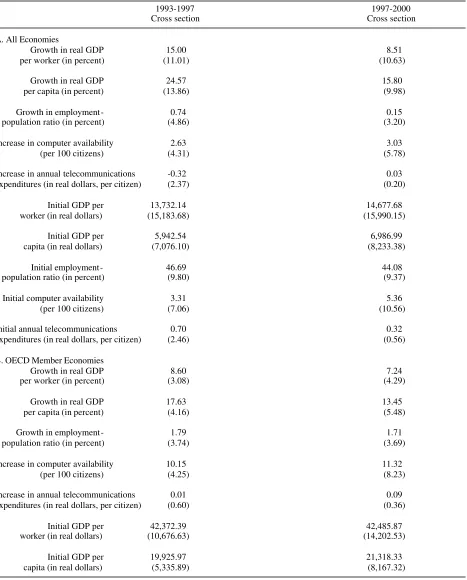
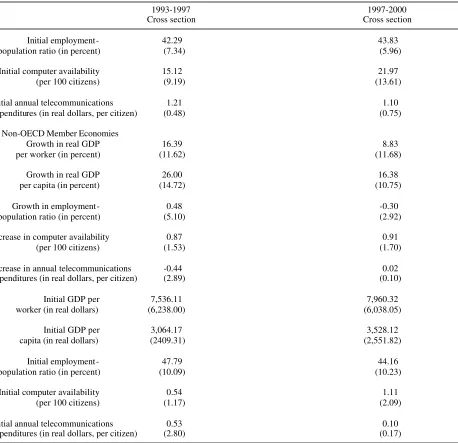
We present the weighted summary statistics for both cross sections in Table 1.5 Using these statistics, we uncover some important trends. First, we note that the availability of personal computers is still very limited globally. Second, the disparity in technology stocks between the developing and developed world is increasing. To highlight these findings, we structure this table into three panels. Panel A presents the summary statistics for all economies that are contained in our two cross sections. Panels B and C contain the statistics for OECD and non-OECD member economies, respectively. Again we use membership in the OECD as our means to distinguish the industrialized from developing economies.

Focusing on Panel A, we see that in both 1993 and 1997, there were fewer than ten computers available for one hundred people to use. In 1993, there were about three computers made ready for each one hundred people to use. By 1997, slightly more than five computers could be used by a group of one hundred people. Investment in technology shrank from being seventy cents per person in 1993 to slightly more than thirty cents in 1997. If we examine the changes in the two technology measures within the two time periods covered by the cross sections, we see universal computer availability is unlikely to be achieved in the near future. The growth in computer availability for both time periods is

5

minuscule. For the last time period contained in our data, only three more computers were made available over a four year time frame.

[Insert Table 1 near here]

Analyzing the growth in economic performance, we see that economic growth slowed over the last half of the 1990s. Worker productivity increased by fifteen percent, with almost twenty- five percent more output was available for consumption at the end of the first five years contained in our data. The respective rates of growth over the 1997 to 2000 time frame were nine and sixteen percent. Growth in the global employment-population ratio was minimal across both time periods. Over neither two periods of time did this measure of economic performance manage to increase in excess one percent.

A comparison of the statistics stylized in Panels B and C uncovers some important trends across the two economy types. Not unexpectedly, we find the OECD member – industrialized economies – have higher initial stocks of computers and higher technology expenditures than do developing economies. Examining the latest data, we see that OECD economies initially had about twenty computers available for use per one hundred citizens. Developing economies provided only one computer per one hundred people for use in 1997. This disparity in computer stocks is also increasing. In both cross sections we see that non-OECD states had significantly fewer computers added to their computer stocks when compared to the industrialized world. A similar trend is evident when we compared investment in telecommunications services across the two economy types.

As expected, we find that the developing world has both lower initial levels of economic output and experiences faster rates of economic growth. This finding is consistent with economic growth theory. Those economies that start out below their steady-state growth paths must grow relatively quickly if they wish to catch up with their peers and growth paths.

estimated coefficients do at least exhibit the expected signs. Taking the first column of Table 2, we can see that having a higher initial level of either worker productivity or computer availability translates into negative growth in worker productivity. The positive, albeit statistically insignificant, coefficient

estimate for increases in the availability of computers suggests that adding an additional computer per one hundred people to an economy’s computer supply increases labor productivity by about 0.14%. We can put this increase into dollar terms using the initial amount of output being produced per worker. At nearly fourteen thousand dollars, each computer added per one hundred citizens equates into each worker producing nineteen dollars’ worth of additional output.

[Insert Table 2 near here]

The results produced in columns 2 and 4 include the two interaction terms. Interestingly, the only statistically findings contained in Table 2 are contradictory. In the 1993-1997 cross section, increased telecommunications investment across all economies served only to reduce labor productivity. However, it would appear that industrialized economies had more success generating a return from this

investment. Each dollar per citizen spent on telecommunications resulted in a higher amount output produced per worker. The growth in labor productivity is of the order of nearly seven percentage points. In the 1997-2001 cross section, however, each dollar spent per citizen by OECD nations actually

decreased labor productivity by almost twelve percentage points. [Insert Table 3 near here]

one hundred citizens increases the per capita real GDP growth rate by almost a full percentage point. In dollar terms, this translates into approximately fifty dollars’ worth of additional output per computer.

The interaction term, however, suggests that any benefit that may be attached to increased computer availability is not to be had within OECD economies. The basic PerComp variable provides us with the general effect that making more computers available holds for per capita GDP. The interaction term between OECD membership and PerComp adjusts this effect to allow for, in this case, a negative differential attached to industrialize status. Therefore, when industrialized economies add a computer to their stocks, the growth rate is reduced by an almost equal magnitude. Each computer added reduces the per capita GDP within industrialized economies by about eight-tenths of one percent.

[Insert Table 4 near here]

Consistent with the findings obtained when we use either per worker or per capita real GDP as the dependent variable, we obtain few significant coefficient estimates when evaluating the

employment-population ratio. The only significant findings of Table 4 are that initial levels of employment are negatively correlated with subsequent increases in ratio of employed persons to an economy’s total population. One explanation for the lack of significant findings in Tables 2 – 4 may be found at the foot of each table. In each cross section, there are fewer than one hundred useable

observations. The analysis of an economy’s employment-population ratio relies on, at best, fewer than fifty observations to generate both the coefficient estimates and their standard errors.

We instead turn to the two panels to see if increased sample sizes lead to more precisely determined results. Unlike the cross section estimation, we cannot include the initial levels of an

dependent to estimate the percentage change in economic growth brought on by a one-unit change in the various dependent variables. Although we present the RE OLS results in Tables 5 – 7, we will limit our discussion to those results that we obtain from the FE OLS specifications. We can still include OECD membership, and the interaction terms, in the FE OLS model given that some economies, notably formerly communist countries, joined this organization at various points in time. Had these

developments not occurred, we would be forced to omit this control from the FE OLS specifications due to collinearity issues.

Table 5 highlights the results of our panel analysis of labor productivity in light of technology changes. Here, we find that each computer added to an economy’s existing computer stock has a

significant, and positive, impact on labor productivity. Each additional computer serves to increase labor productivity by approximately four-tenths of a percentage point. This estimate is found in both the 1993-1997 and 1993-1997-2000 time frames. As was the case in our cross section analyses, when we interact computer availability with membership in the OECD, we find that higher levels of computer availability do not universally increase labor productivity. Within industrialized countries, making available more computers for citizens to use serves to decrease labor productivity by approximately one- half of one percentage point. As a result, there is no benefit to be realized with respect to labor productivity to be realized by industrialized economies increasing the number of available computers.

[Insert Table 5 near here]

It would appear the investment in telecommunications has only recently begun to play a

Turning to the regressions in which we use the log of the annual real per capita GDP, we again see in general technology in general serves to increase the amount of output available for consumption. It is primarily the developing economies that see a benefit attached to increasing their computer

availability and telecommunication investment dollars. Table 6 presents the results of these regressions. Across both periods of time, we see that each additional computer that is added to an economy’s existing supply translates into additional output that is available for consumption. The coefficient estimate of 0.006 implies that each additional computer increases per capita output by approximately six-tenths of one percent. Again, it would appear that OECD economies do not enjoy this increase as they add to their computer stocks. The interaction term between OECD membership and PerComp suggests that each additional computer reduces per capita GDP within industrialized countries by approximately five-tenths of a percentage point.

[Insert Table 6 near here]

As was the case in the cross section, telecommunications expenditures hold conflicting implications for per capita GDP across the two time periods examined here. The coefficient estimate takes on a negative sign over the 1993-1997 time period, but is positively signed for the years between 1997 and 2000. It is only during this later time period that the coefficient estimated for technology investment acquires significance; the estimated coefficient indicates that each dollar spent per person on technology increases per capita GDP in excess of twelve percent. As was the case of greater computer availability, OECD member economies do not seem to enjoy in the beneficial aspects of higher technology expenditures. Each dollar spent on telecommunications spent per person in OECD economies reduces the per capita GDP by eleven percentage points.

[Insert Table 7 near here]

Despite having a larger sample size, very few of the coefficient estimates obtained in our

and investments. In both the cross section and using panel data, we fail to see any significant

relationship between the availability of personal computers or telecommunications investment and the ratio of employed persons. One interpretation of this lack of significance may be that employment levels and, indirectly, unemployment levels are unaffected by the adoption of information technologies.

CONCLUDING REMARKS

Across all estimation techniques and time periods examined, we are guided in the same direction. Technology plays a role in improving labor productivity and the amount of output available for consumption, but only for the developing world. Whatever benefits that the greater availability of computers may have in general, they are lost when incorporated into the industrialized economy’s production function. A similar trend is apparently when evaluating the implications that investment in telecommunications holds for economic performance. Each dollar invested serves to significantly increase both the per worker and per capital GDP, but only for developing economies.

We fail to find any support for, or against, the claim that increased used of information technologies, such as the computer, aggravates the amount of jobless suffered by industrialized

References

[1] Barro, Robert J. and Rachel M. McCleary. “Religion and Economic Growth.” Working Paper #9682, National Bureau of Economic Research, 2003.

[2] Bhagwati, Jagdish, Arvind Panagariya, and T.N. Srinivasan. “The Muddles over Outsourcing.”

Journal of Economic Perspectives, 2004, 18(4), pp. 93 – 114.

[3] Durlauf, Steven, Paul A. Johnson, and Jonathan R. W. Temple. “Growth Econometrics” in Handbook of Growth Economics, Aghion, P. and Durlauf, S. (editors). Amsterdam: North Holland, forthcoming.

[4] Greenwald, Bruce C. and Joseph E. Stigliz. “Labor-Market Adjustments and the Persistence of Unemployment.” American Economic Review, 85(2), pp. 219 – 225.

[5] Heston, Alan and Robert Summers. “The Penn World Table (Mark 5): An Expanded Set of

International Comparison, 1950 – 1988.” Quarterly Journal of Economics, 1991, 106(2), pp. 327 – 68.

[6] Heston, Alan, Robert Summers, and Bettina Aten, Penn World Table Version 6.1, Center for International Comparisons at the University of Pennsylvania (CICUP), October 2002.

[7] International Telecommunications Union. “Yearbook of Statistics: Telecommunications Services 1992 – 2001.” March 2003.

[8] Jovanovic, Boyan. “Growth Theory.” Working Paper #7468, National Bureau of Economic Research, 2000.

Table 1: Weighted Summary Statistics

1993-1997 1997-2000

Cross section Cross section

A. All Economies

Growth in real GDP 15.00 8.51

per worker (in percent) (11.01) (10.63)

Growth in real GDP 24.57 15.80

per capita (in percent) (13.86) (9.98)

Growth in employment- 0.74 0.15

population ratio (in percent) (4.86) (3.20)

Increase in computer availability 2.63 3.03

(per 100 citizens) (4.31) (5.78)

Increase in annual telecommunications -0.32 0.03

expenditures (in real dollars, per citizen) (2.37) (0.20)

Initial GDP per 13,732.14 14,677.68

worker (in real dollars) (15,183.68) (15,990.15)

Initial GDP per 5,942.54 6,986.99

capita (in real dollars) (7,076.10) (8,233.38)

Initial employment- 46.69 44.08

population ratio (in percent) (9.80) (9.37)

Initial computer availability 3.31 5.36

(per 100 citizens) (7.06) (10.56)

Initial annual telecommunications 0.70 0.32

expenditures (in real dollars, per citizen) (2.46) (0.56)

B. OECD Member Economies

Growth in real GDP 8.60 7.24

per worker (in percent) (3.08) (4.29)

Growth in real GDP 17.63 13.45

per capita (in percent) (4.16) (5.48)

Growth in employment- 1.79 1.71

population ratio (in percent) (3.74) (3.69)

Increase in computer availability 10.15 11.32

(per 100 citizens) (4.25) (8.23)

Increase in annual telecommunications 0.01 0.09

expenditures (in real dollars, per citizen) (0.60) (0.36)

Initial GDP per 42,372.39 42,485.87

worker (in real dollars) (10,676.63) (14,202.53)

Initial GDP per 19,925.97 21,318.33

20

Table 1, Continued

1993-1997 1997-2000

Cross section Cross section

Initial employment- 42.29 43.83

population ratio (in percent) (7.34) (5.96)

Initial computer availability 15.12 21.97

(per 100 citizens) (9.19) (13.61)

Initial annual telecommunications 1.21 1.10

expenditures (in real dollars, per citizen) (0.48) (0.75)

C. Non-OECD Member Economies

Growth in real GDP 16.39 8.83

per worker (in percent) (11.62) (11.68)

Growth in real GDP 26.00 16.38

per capita (in percent) (14.72) (10.75)

Growth in employment- 0.48 -0.30

population ratio (in percent) (5.10) (2.92)

Increase in computer availability 0.87 0.91

(per 100 citizens) (1.53) (1.70)

Increase in annual telecommunications -0.44 0.02

expenditures (in real dollars, per citizen) (2.89) (0.10)

Initial GDP per 7,536.11 7,960.32

worker (in real dollars) (6,238.00) (6,038.05)

Initial GDP per 3,064.17 3,528.12

capita (in real dollars) (2409.31) (2,551.82)

Initial employment- 47.79 44.16

population ratio (in percent) (10.09) (10.23)

Initial computer availability 0.54 1.11

(per 100 citizens) (1.17) (2.09)

Initial annual telecommunications 0.53 0.10

expenditures (in real dollars, per citizen) (2.80) (0.17)

Table 2: OLS Estimates of the Change in Real GDP Per Worker [Dependent variable = Percentage Change in Real GDP Per Worker]

1993 – 1997 1997 – 2000

Cross section Cross section

log(Initial GDP -0.527 -0.172 -0.397 -1.414

per worker) (2.413) (2.921) (1.479) (1.673)

Initial computer availability -0.011 -0.007 0.296** 0.206*

(per 100 citizens) (0.252) (0.209) (0.122) (0.119)

Increase in computer 0.140 0.573 0.120** 0.680

availability (per 100 citizens) (0.310) (0.478) (0.051) (0.503)

Initial telecommunications 2.005 -0.358 -2.744 -1.694

investment (per citizen) (2.693) (3.071) (1.999) (2.322)

Increase in telecommunications 2.559 -0.390 0.295 9.950

investment (per citizen) (2.286) (2.978) (1.977) (6.381)

OECD economy 1.338 5.453

(5.308) (4.011)

OECD * Increase in -0.477 -0.598

computer availability (0.528) (0.521)

OECD * Increase in 6.913** -11.677*

telecommunications investment (2.831) (6.305)

n 55 55 81 81

Adjusted R2 0.05 0.10 0.10 0.18

Notes: Results reported at estimated coefficient, (standard error). ***, **, * _{denote significance at the .01, .05 and .10 level,}

22

Table 3: OLS Estimates of the Change in Real GDP Per Capita [Dependent variable = Percentage Change in Real GDP Per Capita]

1993 – 1997 1997 – 2000

Cross section Cross section

log(Initial GDP -0.198 0.187 1.796 0.878

per capita) (3.150) (3.570) (1.961) (2.390)

Initial computer availability -0.135 0.052 0.226 0.175

(per 100 citizens) (0.284) (0.187) (0.173) (0.155)

Increase in computer 0.359 0.886** 0.069 0.638

availability (per 100 citizens) (0.368) (0.414) (0.071) (0.657)

Initial telecommunications 0.799 -2.562 -5.601** -3.408

investment (per citizen) (3.477) (3.721) (2.174) (2.842)

Increase in telecommunications 1.508 -2.641 2.429 15.317

investment (per citizen) (3.135) (3.730) (1.973) (10.822)

OECD economy 2.716 2.263

(5.235) (5.799)

OECD * Increase in -0.837** -0.572

computer availability (0.342) (0.677)

OECD * Increase in 8.053*** -15.223

telecommunications investment (2.972) (10.742)

n 58 58 82 82

Adjusted R2 0.05 0.12 0.08 0.13

Notes: Results reported at estimated coefficient, (standard error). ***, **, * _{denote significance at the .01, .05 and .10 level,}

Table 4: OLS Estimates of the Change in Employment-Population Ratio [Dependent variable = Percentage Change in Employment-Population Ratio]

1993 – 1997 1997 – 2000

Cross section Cross section

log(Initial Employment- -15.096*** -15.387*** -11.340*** -10.568***

Population Ratio) (2.083) (2.124) (3.876) (3.723)

Initial computer availability 0.093 0.008 0.357*** 0.274*

(per 100 citizens) (0.124) (0.146) (0.107) (0.145)

Increase in computer 0.012 0.188 -0.479 -0.486

availability (0.121) (0.156) (0.289) (0.334)

Initial telecommunications 0.143 -1.480 0.651 -0.142

investment (per citizen) (1.329) (1.460) (1.290) (1.542)

Increase in telecommunications 0.806 -1.158 0.558 3.105

investment (per citizen) (1.309) (1.463) (1.598) (5.614)

OECD economy 1.504 3.550

(2.220) (2.616)

OECD * Increase in -0.085 0.020

computer availability (0.139) (0.322)

OECD * Increase in 3.362*** -2.680

telecommunications investment (1.091) (5.865)

n 38 38 49 49

Adjusted R2 0.52 0.58 0.29 0.34

Notes: Results reported at estimated coefficient, (standard error). ***, **, * _{denote significance at the .01, .05 and .10 level,}

24

Table 5: OLS Panel Estimates of Real GDP Per Worker [Dependent variable: Log(Annual Real GDP Per Worker)]

1993 – 1997 1997 – 2000

Panel Panel

Computer availability 0.004*** 0.009*** 0.002*** 0.007*** 0.002*** 0.005*** 0.002*** 0.006***

(per 100 citizens) (0.001) (0.002) (0.001) (0.002) (0.001) (0.003) (0.001) (0.003)

Telecommunications 0.004 0.001 0.003 -0.000 0.024* 0.147*** 0.013 0.086***

investment (per citizen)(0.006) (0.007) (0.006) (0.006) (0.013) (0.033) (0.011) (0.028)

OECD economy 0.073*** 0.034 0.322*** 0.061

(0.028) (0.023) (0.064) (0.057)

OECD * Computer -0.006*** -0.005*** -0.012*** -0.004*

availability (0.005) (0.002) (0.003) (0.002)

OECD * Telecommunications 0.025 0.019 -0.130*** -0.084***

investment (0.017) (0.014) (0.036) (0.030)

FE N N Y Y N N Y Y

n 396 396 396 396 384 384 384 384

Adjusted R2 _{0.26 0.50 0.13 0.35 0.50 0.68 0.43 0.55}

Notes: Results reported at estimated coefficient, (standard error). ***, **, * denote significance at the .01, .05 and .10 level, respectively. All regressions include an intercept and year

Table 6: OLS Panel Estimates of Real GDP Per Capita [Dependent variable: Log(Annual Real GDP Per Capita)]

1993 – 1997 1997 – 2000

Panel Panel

Computer availability 0.004*** 0.010*** 0.002** 0.006*** 0.002*** 0.017*** 0.001 0.006**

(per 100 citizens) (0.001) (0.002) (0.001) (0.002) (0.001) (0.003) (0.001) (0.003)

Telecommunications -0.004 -0.002 0.002 -0.003 -0.039*** 0.207*** 0.022* 0.119***

investment (per citizen)(0.007) (0.008) (0.006) (0.006) (0.014) (0.035) (0.012) (0.029)

OECD economy 0.063** 0.019 0.443*** 0.094

(0.028) (0.021) (0.069) (0.061)

OECD * Computer -0.006*** -0.005*** -0.015*** -0.005*

availability (0.002) (0.002) (0.003) (0.003)

OECD * Telecommunications 0.032 0.025* -0.180*** -0.113***

investment (0.019) (0.015) (0.039) (0.032)

FE N N Y Y N N Y Y

n 409 409 409 409 388 388 388 388

Adjusted R2 _{0.16 0.40 0.05 0.13 0.44 0.72 0.24 0.50}

Notes: Results reported at estimated coefficient, (standard error). ***, **, * denote significance at the .01, .05 and .10 level, respectively. All regressions include an intercept and year

26

Table 7: OLS Panel Estimates of Employment-Population Ratio [Dependent variable: Log(Annual Employment-Population Ratio)]

1993 – 1997 1997 – 2000

Panel Panel

Computer availability -0.001 -0.000 -0.001* -0.001 0.000 -0.001 -0.000 -0.004*

(per 100 citizens) (0.001) (0.001) (0.001) (0.001) (0.000) (0.002) (0.000) (0.002)

Telecommunications 0.006* 0.005 0.006* 0.005 0.016** 0.003 0.010 -0.014

investment (per citizen)(0.004) (0.004) (0.004) (0.004) (0.007) (0.018) (0.007) (0.018)

OECD economy -0.005 -0.015 0.017 -0.090**

(0.013) (0.013) (0.030) (0.035)

OECD * Computer -0.001 -0.000 0.001 0.004**

availability (0.001) (0.001) (0.002) (0.002)

OECD * Telecommunications 0.009 0.007 0.015 0.024

investment (0.009) (0.009) (0.019) (0.019)

FE N N Y Y N N Y Y

n 249 249 249 249 259 259 259 259

Adjusted R2 0.00 0.00 0.08 0.10 0.24 0.24 0.00 0.15

Notes: Results reported at estimated coefficient, (standard error). ***, **, * _{denote significance at the .01, .05 and .10 level, respectively. All regressions include an intercept and year}