A multi agent growth model based on the von Neumann Leontief framework

Munich Personal RePEc Archive

A multi-agent growth model based on

the von Neumann-Leontief framework

Li, Wu

College of International Business and Management, Shanghai

University

8 August 2008

Online at

https://mpra.ub.uni-muenchen.de/11302/

A Multi-Agent Growth Model Based on

the von Numann-Leontief Framework

LI WU

*

College of International Business and Management, Shanghai University, P.R.C.

ABSTRACT This paper presents a discrete-time growth model to describe the dynamics of a multi-agent economy, and the model consists of production process, exchange process, price and technology adjustment processes etc. Technologies of agents in each period are represented by a technology matrix pair, and some properties of Perron-Frobenius eigenvalues and eigenvectors of technology matrix pairs are discussed. An exchange model is also developed to serve as the exchange part of the growth model. And equilibrium paths of the growth model are proved to be balanced growth paths sharing a unique normalized price vector. Though this paper focuses mainly on the case of n agents and n goods, the growth model can also deal with the case of m agents and n goods. A numerical example with 6 agents and 4 goods is given, which describes the dynamics of a two-country economy and has endogenous price fluctuations and business cycles.

KEY WORD: von Neumann’s expanding economic model, input-output model, dynamic general equilibrium, disequilibrium, multi-country economic model

1. Introduction

The expanding economic model of von Neumann (1945) and the input-output model of Leontief (1936, 1941) laid the foundation of a distinct modern framework for economic analysis. And the von Neumann-Leontief framework is greatly enriched and improved by Kemeny, Morgenstern and Thompson (1956), Gale (1956, 1960), Dorfman, Samuelson and Solow (1958), Morishima (1960, 1964), Sraffa (1960), McKenzie(1963, 1976), and numerous other works including some recent ones such as the studies on stochastic von Neumann–Gale model by Dempster, Evstigneev and Taksar (2006), and Evstigneev and Schenk-Hoppe (2007).

The von Neumann-Leontief framework provides a deep insight into the structure and interdependency of all parts of the economy, and furnishes proper tools to explore both the nature of economic structure and the dynamic general equilibrium. Until now, however, some major economic

elements haven’t been incorporated explicitly into the framework, e.g. maximizing agents, exchange process among agents, price fluctuation and technology adjustment etc. This paper aims to combine some fundamental thoughts of the von Neumann-Leontief framework with those elements mentioned above by developing a new growth model.

As the expanding economic model of von Neumann (1945), the growth model in this paper treats the economy as a discrete-time dynamic system. Matrix pairs are also used to represent technologies adopted by agents in each period, and as a consequence durables goods can be treated in the form of joint production.

On the other hand, unlike the expanding economic model which in fact consists of a set of equilibrium conditions, no equilibrium condition is presumed when building the growth model in this paper. That is, whether there exists an equilibrium or not, the growth model here is workable. In fact, the model is an autonomous system focusing on describing decision-making processes and interactions of maximizing agents under changing economic circumstances which generally are in disequilibrium. In this sense the growth model here is in essence a disequilibrium one, though the equilibrium paths of the model are still analyzed in this paper.

The paper is organized as follows. Section 2 and 3 discuss the representation method of technologies and some properties related to technology matrix pairs. Section 4 presents an exchange model. Section 5 introduces the growth model, which contains the exchange model as a part. Section 6 is devoted to the equilibrium analysis of the growth model. Section 7 presents a numerical example with m agents and n goods. And the final section contains some open discussions.

2. Technology Matrix Pairs

Analogous to input-output models, we start with an economy including n agents and n goods which are indexed by 1, 2,×××,n, and good i is produced only by agent i. Each agent attempts to maximize its profit (i.e. minimize its cost). Such an agent may stand for a firm or a sector. If we regard a household as a producer of labor power (or human capital, service, etc.), which absorbs consumer goods, education, trainings and medical treatment etc, and regard its consumption process as an investment and production process, then such an agent can also stand for a household roughly. And such treatment of the consumption process is generally used in the so-called closed models based on the von Neumann-Leontief framework (e.g., see Solow and Samuelson, 1953).

In the sequel the following notations and terms will be used. 0 denotes a zero vector or zero matrix, and e denotes the vector (1, 1,_×××, 1)T

. A vector x is called nonnegative (or positive) and we write x³0 (or x_0) if all its components are nonnegative (or positive). x is called semipositive and we write x>0 if x³0 and x¹0. A semipositive column (or row) vector x is said to be normalized if e xT =1 (or xe=1) holds. For vectors x and y, we write xy, x>y and x³ y

matrices.

2.1. Production and Technology

We regard the economy as a discrete-time dynamic system, and in each period of the economy the production process of an agent is an input-output process which absorbs an input bundle a and yields an output bundle b. Hence a feasible production process of an agent can be represented by a

n-dimensional column vector pair ( , )a b .

For a production process ( , )a b of agent i, if the input bundle is used up in the production, the output bundle contains only good i as the product, that is, b_k =0 holds for all k¹i, where b_k

denotes the kth component of b. In order to take account of durable goods or capital goods, let’s suppose after production some input goods may have remainders. Thus the output bundle b now may contain both one kind of product and some remainders of input goods, and may have more than one positive component. The assumptions on production processes of each agent are summarized as follows.

Assumption 2.1: Let ( , )a b be a feasible production process of agent i, then: (i) if ( , )a b ¹( , )0 0 then a>0 and b>0 hold;

(ii) if k¹i and a_k >0 then b_k <a_k; if k¹i and a_k =0 then b_k =0; (iii) for any xÎ₊,

(

xa, xb

)

is also a feasible production process of agent i.

Assumption 2.1 implies every input good will undergo depreciation more or less in production, and production has constant returns to scale.

Definition 2.1: Let ( , )a b be a feasible production process of agent i. If bi =1 then ( , )a b is called a technology of agent i, and a is called a standard input bundle of agent i; moreover, for a production process

(

xa, xb

)

, xÎ+, x is called the production intensity of the production

process.

By the definition above, a technology is a feasible production process with a unit of production intensity, which needs one standard input bundle as inputs.

We make the following assumption on technologies to simplify the analysis.

Assumption 2.2: Each agent possesses at least one and at most finitely many technologies.

2.2. Technology Matrix Pairs

Definition 2.2: A n-by-n matrix pair

(

A B,

)

is called a technology matrix pair (TMP), if

(

( ) ( )

)

,

i i

a b is a technology of agent i for all i=1, 2,×××,n, where ( )i

a and ( )i

b denote the ith columns of A and B respectively; moreover, A and B are called an input coefficient matrix and

output coefficient matrix respectively. A TMP

(

A B,

)

is called a minimal cost rate TMP under a price vector p, if

(

( ) ( )

)

,

i i

a b is a minimal cost rate technology of agent i under p for all 1, 2, ,

i= ×××n. A TMP

(

A B,

)

is said to be productive if there is a semipositive vector x such that

Ax£Bx.

Let T denote the set of all TMPs, then by Assumption 2.2 there are a finite number of TMPs in

T. For TMPs, we make the following assumption.

Assumption 2.3: There is at least a productive TMP in T; and for each TMP

(

A B,

)

Î T, the input coefficient matrix A is indecomposable.

The existence of productive TMP provides the possibility of growth. And the indecomposability of each input coefficient matrix guarantees that every good is indispensable in a growing economy.

By Assumption 2.1, 2.3 and Definition 2.1, it’s clear that each TMP

(

A B,

)

Î T can be written as

(

A I, +R

)

such that R is nonnegative and A R- is nonnegative and indecomposable.

2.3. Perron-Frobenius Eigenvalues and Eigenvectors of TMPs

For an indecomposable nonnegative square matrix M, let r(M) denote its spectrum radius. And the following lemma is a well-known result of Perron-Frobenius theorem (e.g., see Debreu and Herstein, 1953).

Lemma 2.1: Let M be an indecomposable nonnegative square matrix, x be a semipositive column vector and aÎ, then:

(i) Mx£axÞr(M)£a;Mx<axÞr(M)<a;

(ii) T T ( )

x M£ax Þr M £a; T T ( )

x M<ax Þr M <a.

By Lemma 2.1 some necessary and sufficient conditions for the productivity of TMPs can be obtained, as the following lemma shows.

Lemma 2.2: For each TMP

(

A B,

)

Î T, the following statements are equivalent: (i)

(

A B,

)

is productive;

(ii) r(A R- ) 1£ , where Rº -B I;

(iii) there is a semipositive vector yT such that y AT £y BT .

semipositive vector x such that Ax£Bx, that is,

(

A R x-

)

£x. Since A R- is nonnegative and indecomposable, by Lemma 2.1(i) we find r(A R- ) 1£ .

Secondly, let’s prove (ii) implies (iii). Suppose r(A R- ) 1£ holds, then by Perron-Frobenius theorem there is a positive vector yT such that yT(A R- )=lyT, where l=r(A R- ). Thus we find yT(A R- )£ yT, that is, y AT £ y BT .

Finally, let’s suppose (iii) holds. By Lemma 2.1(ii) we find r(A R- ) 1£ . Then by

Perron-Frobenius theorem it_’s clear that

(

A B,

)

is productive. █

Some results of Perron-Frobenius theorem have been extended to matrix pairs by Mangasarian (1971), Bapat, Olesky and van den Driessche (1995), Mehrmann, Nabben and Virnik (2008). Here let’s define the Perron-Frobenius eigenvalues and eigenvectors of semipositive square matrix pairs as follows.

Definition 2.3: Let

(

A B,

)

be a semipositive square matrix pair. If there exist a positive real number l and two positive vectors T

y and x such that Ax=lBx and T T

y A=ly B, then l, T

y and x are called the P-F (i.e. Perron-Frobenius) eigenvalue, left and right P-F eigenvectorof

(

A B,

)

respectively; and in the special case B=I, they are also called the P-F eigenvalue, left

and right P-F eigenvectorofA respectively.

The following lemma stems from Bapat, Olesky and van den Driessche (1995).

Lemma 2.3: For a semipositive square matrix pair

(

A B,

)

, if B-A is nonsingular and

1

(B-A)- A is nonnegative and indecomposable, then

(

A B,

)

possesses a unique P-F eigenvalue (0,1)

lÎ , a unique normalized left P-F eigenvector and a unique normalized right P-F eigenvector.

Lemma 2.4: Each productive TMP

(

A B,

)

Î T possesses a unique P-F eigenvalue lÎ(0,1], a unique normalized left P-F eigenvector and a unique normalized right P-F eigenvector.

Proof. Let Rº -B I. Since

(

A B,

)

is productive, by Lemma 2.2 we find r(A R- ) 1£ . First let_’s consider the case r(A R- ) 1< . It_’s well known that 1

1

( ) k

k

I M I M

¥

-=

- = +

å

holds for

any square matrix M satisfying r(M) 1< (e.g., see Horn and Johnson, 1990). So we have

1

1

( ) ( )k

k

B A I A R I

¥

-=

- = +

å

- > ,

then 1

(B-A)- A> A holds. Since A is nonnegative and indecomposable, it_’s clear that 1

(B-A)- A

is nonnegative and indecomposable. By Lemma 2.3 the statement holds. If r(A R- )=1 holds, let T

y and x denote the normalized left and right P-F eigenvectors of

A R- respectively, then by Perron-Frobenius theorem it_’s clear that T T

y A=y B and Ax=Bx

holds. That is,

(

A B,

)

has the P-F eigenvalue 1. If

(

A B,

)

has any other P-F eigenvalue l, then there is a positive vector _y¢T

such that T T

y A¢ =ly B¢ . By T T

y Ax¢ =ly Bx¢ and T T

the P-F eigenvalue 1 is also a left (or right) P-F eigenvector of A R- , by Perron-Frobenius theorem we find yT and x are the unique normalized left and right P-F eigenvectors of

(

A B,

)

respectively. Hence the statement holds. █

If a non-productive TMP possesses a P-F eigenvalue l, by the definitions of productive TMP and P-F eigenvalue we can see that l>1 holds.

Some properties of the P-F eigenvalues and eigenvectors of matrices are also retained in the case of matrix pairs. For instance, the following lemma is an extension of Lemma 2.1.

Lemma 2.5: Let

(

A B,

)

be a semipositive square matrix pair possessing a P-F eigenvalue l, and A is indecomposable. Let x be a semipositive vector and aÎ. Then:

(i) Ax<aBxÞ <l a;Ax£aBxÞ £l a; (ii) Ax>aBxÞ >l a;Ax³aBxÞ ³l a;

(iii) T T

x A<ax BÞ <l a; T T

x A£ax BÞ £l a; (iv) _{x A}T _{x B}T

a l a

> Þ > ;_{x A}T _{x B}T

a l a

³ Þ ³ .

Proof. (i) Let T

y be a left P-F eigenvector of

(

A B,

)

such that T T

y A=ly B. Since T

y is positive, we have:

T T T T

Ax<aBxÞy Ax<ay BxÞly Ax<ay Ax. Since A is indecomposable, it_’s clear that T 0

y Ax> , thus we find l<a.

The rest of the proof is analogous. █

3. Optimal Technology Matrix Pairs

This section is devoted to the analysis of some properties related to the minimal P-F eigenvalue of productive TMPs, and conclusions will be used in the equilibrium analysis of Section 6.

Definition 3.1: Among all productive TMPs belonging to T, a TMP possessing the minimal P-F eigenvalue is called an optimal technology matrix pair (optimal TMP), and the minimal P-F eigenvalue is denoted by *

l .

By Assumption 2.2, Assumption 2.3 and Lemma 2.4, there exists at least one optimal TMP, and

* ₁

l £ holds.

Lemma 3.1: Let pT be a left P-F eigenvector of an optimal TMP, then:

(i) T * T

p a³l p b holds for each technology ( , )a b of each agent; (ii) p AT ³l*p BT holds for each TMP ( , )A B Î T.

Proof. (i) Suppose T

p is a left P-F eigenvector of the optimal TMP ( ,A B¢ ¢) , then

*

T T

p A¢=l p B¢. If agent i has a technology ( , )a b such that T * T

ith columns of A¢ and B¢ with a and b respectively we obtain a new TMP

(

A B¢¢ ¢¢ Î T,

)

satisfying p AT ¢¢<l*p BT ¢¢. By * ₁

l £ and Lemma 2.2,

(

A B¢¢ ¢¢,

)

is productive, and by Lemma 2.4

(

A B¢¢ ¢¢,

)

has a P-F eigenvalue l¢¢. By p AT ¢¢<l*p BT ¢¢ and Lemma 2.5(iii) we find *

l¢¢ <l . Recall the definition of *

l , there is a contradiction. Hence the statement holds.

(ii) It_’s an immediate result of (i). █

The following proposition shows the normalized left P-F eigenvector of optimal TMPs is unique.

Proposition 3.1: All optimal TMPs share the same normalized left P-F eigenvector.

Proof. Let

(

A B,

)

and

(

A B¢ ¢,

)

be two optimal TMPs, which possess the P-F eigenvalue *

l . Let T

p denote the normalized left P-F eigenvector of

(

A B,

)

. By Lemma 3.1(ii) we find T * T

p A¢³l p B¢. If T * T

p A¢>l p B¢ holds then by Lemma 2.5(iv) we find the absurdity * *

l >l . Thus T * T

p A¢=l p B¢ must hold, that is, T

p is the normalized left P-F

eigenvector of

(

A B¢ ¢,

)

. █

3.1. Minimal Cost Rates of Agents

Obviously, given a price vector p the potential profit rate level of each agent depends on its minimal cost rate under p. As for minimal cost rates of agents, we have the following proposition.

Proposition 3.2: Let p be a positive price vector, either (i) or (ii) holds: (i) minimal cost rates of all agents under p equals *

l ;

(ii) there is an agent whose minimal cost rate under p is greater than *

l , and there is another agent whose minimal cost rate under p is smaller than *

l .

Proof. If the minimal cost rate of each agent under p is no smaller than *

l and there is an agent whose minimal cost rate under p is greater than *

l , then for any

(

A B,

)

Î T ,

*

T T

p A>l p B holds. Let

(

A B¢ ¢,

)

be an optimal TMP. By p AT ¢>l*p BT ¢ and Lemma 2.5(iv) we find * *

l >l . There is a contradiction.

If the minimal cost rate of each agent under p is no greater than *

l and there is an agent whose minimal cost rate under p is smaller than *

l , then there is a TMP

(

A B,

)

Î T such that

*

T T

p A<l p B. By Lemma 2.2,

(

A B,

)

is productive. Furthermore, by Lemma 2.4 and Lemma 2.5(iii)

(

A B,

)

has a P-F eigenvalue smaller than *

l , which contradicts the definition of *

l .

Henceeither (i) or (ii) holds. █

Proposition 3.2 implies under any positive price vector there is an agent whose minimal cost rate is no greater than *

l .

Proof. Let l denote the P-F eigenvalue of

(

A B,

)

such that p AT =lp BT , then under p the cost rate of each technology in

(

A B,

)

equals l.

First let’s suppose

(

A B,

)

is a minimal cost rate TMP under p, then for any productive TMP ( ,A B¢ ¢ Î T) with a P-F eigenvalue l¢ we have p AT ¢³lp BT ¢, and by Lemma 2.5(iv) we find

l¢ ³l. Hence *

l=l holds and

(

A B,

)

is an optimal TMP.

Now let’s suppose

(

A B,

)

is an optimal TMP, then under p the cost rate of each technology in

(

A B,

)

equals *

l .By Lemma 3.1(ii)

(

A B,

)

is a minimal cost rate TMP under p. █

3.2. Convex Combination of TMPs

In this paper the convexity of the technology set of each agent is not assumed. And the following proposition and the analysis in the sequel indicate that the convexity assumption on technology sets is relatively unimportant.

Proposition 3.4: Let ( ,A B) be a convex combination of k TMPs, that is, ( ) ( ) 1

k i i

i

A a A =

=

å

and

( ) ( ) 1

k i i

i

B a B =

=

å

where ( ) ( )

1

, 1

k

i i

i

a ₊₊ a

=

Î_

å

= ,

(

A( )i ,B( )i

)

Î T. If ( ,A B) has a P-F eigenvalue l,

then *

l³l holds.

Proof. Let T

p be a left P-F eigenvector of an optimal TMP. Then by Lemma 3.1(ii) we find:

( ) ( ) * ( ) ( ) *

1 1

k k

T i T i i T i T

i i

p A a p A l a p B l p B

= =

=

å

³

å

= .

Note that A is indecomposable, by Lemma 2.5(iv) the statement holds. █

Analogously we can also find that a convex combination of optimal TMPs must possess the P-F eigenvalue *

l .

4. An Exchange Model

This section is devoted to the exchange process among n agents. And a short-term exchange model will be presented, in which both the price vector and each agent_’s demand structure are fixed. Under some reasonable assumptions we will find the model has a unique exchange result. And the model will play a part in the growth model in Section 5.

Suppose the exchange process occurs among n agents and under a given price vector p, in which each agent sells its outputs and purchases its standard input bundle for production.

Let S denote the supply matrix, whose ( , )i j entry denotes agent j_’s supply amount of good i. Let sºSe denote the supply vector, which is supposed to be positive.

Demand structures of agents are represented by a given input coefficient matrix A and each agent intends to purchase some standard input bundles indicated by A for its production. That is, in the exchange process the bundle purchased by agent i must be ( )i

a

column of A. x is called the purchase amount of agent i. Let z denote the vector consisting of purchase amounts of n agents, and z is called the purchase vector or exchange vector.

Obviously, the ( , )i j entry of Az indicates agent j’s purchase amount of good i, and the total purchase amount of n goods can be represented by Az. Here we write x to denote diag(x), i.e. the diagonal matrix with the vector x as the main diagonal. Though diag(x) is the generally used notation, considering it’s much frequently used in this paper we adopt the new notation to make formulas clearer and shorter.

The sales rate of a good refers to the proportion of its sales amount to its supply amount. Suppose for one good all its suppliers share the same sales rate. And let u be the n-dimensional sales rate vector indicating the sales rates of n goods. Then the total sales amounts of n goods are us . And the following equation holds obviously.

Az=us (4.1)

(4.1) means the balance of material in the exchange process, that is, the total purchase amount of each good equals its total sales amount. And (4.1) can also be written as u=s Az-1 .

On the other hand, under the given price vector p, the purchase and sales values of n agents are T

p Az and T

p uS respectively. And the value each agent purchases must equal the value it sells, that is:

T T

p Az=p uS (4.2)

(4.2) means the balance of value in the exchange process. By (4.1) and (4.2), we obtain:

1

T T

p Az=p s AzS- (4.3)

When (4.3) holds and T

S A is indecomposable, the following proposition shows that there exists a unique normalized exchange vector.

Proposition 4.1: Let A and S be n-by-n semipositive matrices such that sºSe is positive and T

S A is indecomposable. Let p be an n-dimensional positive vector and z be an n -dimensional semipositive vector. Then:

(i)  

1 ₁

T T

Z A p S s pA -

-º  is an indecomposable nonnegative matrix possessing the P-F

eigenvalue 1;

(ii) z satisfies T T1

p Az= p s AzS- if and only if z is a right P-F eigenvector of Z ; (iii) if z satisfies T T1

p Az= p s AzS- then z is positive.

Proof. (i) Because _{S A}T

is indecomposable, each column of A must be semipositive. Then A pT

is a positive vector, and all entries on the main diagonals of 

1

T

A p

-, s-1 and p are positive. Hence if the

( )

i j, entry of _{S A}T

is positive then the

( )

i j, entry of Z is also positive. Therefore

Z is indecomposable.

eigenvalue of Z equals 1 and p AT is a left P-F eigenvector of Z. (ii) We have:

1 _ 1 _ 1

T T T T T T

p Az=p s AzS- Û p Az= p Azs S- ÛA pz=S s pAz - 1 ₁

T T

A p S s pAz z Zz z -

-Û  = Û = .

Hence by Perron-Frobenius theorem the statement holds.

(iii) It_’s an immediate result of (ii). █

Let z¢ denote the normalized right P-F eigenvector of Z, then by Proposition 4.1(ii) we have

z=xz¢, where xÎ+. Since the sales amount of each good is no more than its supply amount, we

find Az£s holds, that is, xAz¢ £s holds. Hence x is no greater than the minimal component of Az¢-1s. Suppose all agents attempt to obtain maximal exchange amounts. The unique maximal exchange vector can be found by following steps, which stands for the exchange result of the exchange process:

STEP 1. Compute the matrix  

1 ₁

T T

Z A p S s pA -

-º  ;

STEP 2. Find the normalized right P-F eigenvector of Z , denoted by z¢; STEP 3. Find the minimal component of Az¢-1s, denoted by x;

STEP 4. Compute the exchange vector zºxz¢.

Thus the exchange process can be represented by a function as follows:

(

u z,

)

=Z

(

A p S, ,

)

(4.4)

where A, S and p satisfy those assumptions in Proposition 4.1, and z is computed by steps above and

u equals s Az-1 . Here we write u explicitly on the left side of (4.4) only for the expression convenience of the growth model in Section 5. Since T

S A is supposed to be indecomposable, accordingly the exchange process above is said to be an indecomposable exchange process.

In the discussion so far, some stringent assumptions are made on the exchange process, and those assumptions may be relaxed. Here let’s discuss two cases briefly.

First, when A and S are n-by-m matrices, it’s clear that the results of Proposition 4.1 also holds. That is, without essential modification the discussion in this section can also be applied to the case of m agents and n goods.

Second, when T

S A is decomposable, we will find that agents involved in the exchange process can be divided into some groups to exchange independently, that is, the exchange process can be divided into some independent and indecomposable exchange processes. Hence the analysis of the decomposable case will be analogous, and eventually we can also obtain a unique exchange vector.

5. The Growth Model

period. And the state of the economy in period t is represented by following variables:

p(t) Price vector, which is positive and consists of prices of n goods in period t;

(

( ) ( )

)

,

t t

A B TMP, which represents those technologies adopted by agents in period t;

( )t

S Supply matrix, whose

( )

i j, entry stands for the agent j’s supply amount of good i in period t;

( )t

u Sales rate vector, which consists of sales rates of n goods in period t;

( )t

z Exchange vector and production intensity vector, which represents the amounts of standard input bundles that are purchased and put into production by agents in period t;

( )t

Y Output matrix, whose

( )

i j, entry stands for the output amount of good i by agent j in period t.

Suppose in period t+1 the economy runs as follows.

Firstly, the new price vector emerges on the basis of the price vector and sales rates of period t, which indicates the market prices of n goods in period t+1.

Secondly, each agent adjusts its technology according to the new price vector to maximizing its profit rate, and the new TMP is formed.

Thirdly, outputs and depreciated inventories of period t constitute the supplies in period t+1. Fourthly, supplies are exchanged under market prices, and the exchange vector and sales rates vector of period t+1 are obtained. Unsold goods constitute the inventories of period t+1, which will undergo depreciation and become a portion of the supplies of next period.

Finally, each agent puts into production its input bundle purchased in the market, and outputs of period t+1 are obtained.

The growth model is as follows:

(

)

( 1) ( ) ( )

,

t t t

p + =P p u (5.1)

(

( 1) ( 1)

)

(

(

( ) ( )

)

( 1)

)

, , ,

t t t t t

A + B + =H A B p + (5.2)



(

)

(t 1) ( )t ( )t ( )t

S + =Y +Q e u S- (5.3)

(

( 1) ( 1)

) (

( 1) ( 1) ( 1)

)

, , ,

t t t t t

u + z + =Z A + p + S + (5.4)

 (t 1) (t 1) (t 1)

Y + =B + z + (5.5)

Let _x( )t

denote

(

( )

(

( ) ( )

)

( ) ( ) ( ) ( )

)

, , , , , ,

t t t t t t t

p A B S u z Y . A path of the model (5.1)-(5.5) is denoted by a sequence

{ }

( )

0

t t

x ¥ = .

Let’s explain equations in the model in turn. Meanwhile some assumptions will be made to facilitate the equilibrium analysis of the model.

Assumption5.1: The price adjustment function p=P

(

p u¢,

)

satisfies: u= Ûe p= p¢.

That is, if and only if all goods clear the price vector won’t change. (5.2) stands for the technology adjustment process, and : n

+ + T´ ® T

H _ is the technology

adjustment function, which stands for the process that each agent adjusts its technology according to market prices to minimize its cost rate. And the ith columns of input and output coefficient matrices are adjusted by agent i. For the technology adjustment function the following assumption is made.

Assumption 5.2: The technology adjustment function

(

A B,

)

=H

(

(

A B¢ ¢,

)

,p

)

satisfies:

(

A B,

)

is equal to

(

A B¢ ¢,

)

if and only if

(

A B¢ ¢,

)

is a minimal cost rate TMP under p.

That is, no agent adjusts its technology if and only if the old TMP is a minimal cost rate TMP under the current price vector.

(5.3) stands for the formation of supplies. If ( )t

u ¹e, then there are some unsold goods in period

t. The inventory amounts of agents in period t are indicated by the inventory matrix ( )t ( )t

e u S- . Q is the inventory depreciation function, which stands for the depreciation process of inventories and is defined on the nonnegative matrix set, and the following assumption is made.

Assumption 5.3: For any nonnegative matrix M, 0£Q

( )

M £M holds.

The outputs of period t, which is denoted by ( )t

Y , plus the depreciated inventories of period t, which is denoted by

(

( )t ( )t

)

e u S

-Q , forms the supplies of period t+1, which is denoted by (t 1) S + . (5.4) stands for the exchange process, and Z is the exchange function obtained in Section 4. Let’s make the following assumption to guarantee that each agent possesses initial endowment.

Assumption 5.4: _z(0)

0

 holds. Note that T

B A³A holds for each TMP

(

A B,

)

Î T, by Assumption 2.3 we find T

B A is indecomposable for each

(

A B,

)

Î T. Since (0)

z is positive, by (5.5), (5.3) and Proposition 4.1(iii) it_’s clear that ( )t T ( )t

S A is indecomposable and ( )t

z _0 holds for all t=1, 2,_,¥. (5.5) stands for the formation of outputs. Since (t 1)

i

z + indicates the amount of the standard input bundle purchased by agent i in period t+1 and a standard input bundle corresponds to a unit of productivity intensity, (t 1)

i

z + also indicates the productivity intensity of agent i in period t+1. We write (5.5) explicitly in the model only for clarity. (5.5) can be omitted if (5.3) is written as follows:



(



)

(t 1) ( )t ( )t ( )t ( )t

S + =B z +Q e u S- ( 5.3¢)

6. Equilibrium Paths

Definition 6.1: A path of the model (5.1)-(5.5) is called an equilibrium path if it satisfies: (i)

( )t

u =e; (ii)

(

( ) ( )

) (

(0) (0)

)

, ,

t t

A B = A B , for all t=0,1, 2,××× ¥, .

The first equilibrium condition says that in an equilibrium path all goods clear all the time. By the assumption on the price adjustment function, i.e. Assumption 5.1, this condition implies that the price vector keeps constant all the time. That is, in an equilibrium path ( )t (0)

p = p holds for all

0,1, 2, ,

t= ××× ¥, and (0)

p is called an equilibrium price vector.

The second equilibrium condition says that in an equilibrium path the TMP keep constant all the time, and the TMP is called an equilibrium TMP. By the assumption on the technology adjustment function, i.e. Assumption 5.2,

(

(0) (0)

)

,

A B must be a minimal cost rate TMP under the equilibrium price vector so that each agent needn’t adjust its technology.

And the following lemma is immediate.

Lemma 6.1: Let

{ }

( ) 0

t t

x ¥

= be an equilibrium path of the model (5.1)-(5.5), in which the

equilibrium TMP and the equilibrium price vector are

(

A B,

)

and p respectively, then the equilibrium path satisfies:

(i) ( )

(

(

)

( 1) ( ) ( )

)

, , , , , ,

t t t t

x = p A B Bz - e z Bz holds for all t=1, 2,××× ¥, ; (ii)

(

( 1)

)

(

( )

)

, t , , t

e z + =Z A p B z holds for all t=0,1, 2,××× ¥, ; (iii) (t 1) ( )t

Az + =Bz holds for all t=0,1, 2,××× ¥, ; (iv) T (t 1) T ( )t

p Az + =p Bz holds for all t=0,1, 2,××× ¥, ; (v)

(

A B,

)

is a minimal cost rate TMP under p.

Equilibrium paths of models based on the von Neumann-Leontief framework are always closely related with balanced growth paths. The growth model in this paper is no exception, even though equilibrium paths here are defined in a distinct way. Here we define balanced growth paths as follows.

Definition 6.2: Let

(

A B,

)

be an optimal TMP and

{ }

( ) 0

t t

x ¥

= be a path of the model (5.1)-(5.5).

{ }

( ) 0

t t

x ¥

= is called a balanced growth path corresponding to

(

A B,

)

if it satisfies:

(i)

(

A( )t ,B( )t

)

=

(

A B,

)

holds for all t=0,1, 2,××× ¥, ;

(ii) z(0) is a right P-F eigenvector of

(

A B,

)

and _z( )t * t_z(0)

l

-= holds for all

0,1, 2, ,

t= ××× ¥; (iii) (0)T

p is a left P-F eigenvector of

(

A B,

)

and ( )t (0)

p = p holds for all t=0,1, 2,××× ¥, .

By Proposition 3.3, we find that in a balanced growth path corresponding to an optimal TMP

(

A B,

)

,

(

A B,

)

is the minimal cost rate TMP under the price vector of any period. Furthermore, it can be readily verified that a balanced growth path corresponding to an optimal TMP is an equilibrium path.

growth path corresponding to an optimal TMP.

Proposition 6.1: Let

{ }

( )

0

t t

x ¥

= be an equilibrium path of the model (5.1)-(5.5), in which the

equilibrium TMP and the equilibrium price vector are

(

A B,

)

and p respectively, then the equilibrium path satisfies:

(i) ( )t * t (0)

z =l -z holds for all t=0,1, 2,××× ¥, ; (ii)

(

A B,

)

is an optimal TMP; moreover, T

p and (0)

z are its left and right P-F eigenvectors respectively.

Proof. (i) From Lemma 6.1(iv) we have:

     1

( 1) ( ) ( 1) ( ) ( 1) ( )

T t T t T t T t t T T t

p Az p B z p Az p Bz z p A p Bz -+ _{= Þ} + _{= Þ} + ₌

.

Let 

1

T T

g p A p B

-º , so (t 1)  ( )t

z + =gz .

Since

(

A B,

)

is a minimal cost rate TMP under p, 1g_i is the minimal cost rate of agent i under

p for all i=1, 2,×××,n. Denote the maximal component of g by x, then by Proposition 3.2 * 1

x ³l

-holds.

If all components of g are same, then by Proposition 3.2 we find * 1

g=l -e and the statement holds.

Now let’s suppose some component of g is smaller than x. From Lemma 6.1(iii) we have:

 1   1 

(t 1) ( )t t (0) t (0) t 1 t (0) t 1 t (0)

Az + =Bz ÞAg +z =Bg z ÞAx- - g +z =Bx- - g z .

Let

(

 (0)

)

lim t t t

z x- g z ®¥

¢ º , then z¢ must be a semipositive vector containing at least one zero

component, and 1

Az¢=x-Bz¢ must hold. Hence we find:

(

xA R z-

)

¢=z¢,

where Rº -B I.

By * 1

1

x ³l- ³ , xA-R is nonnegative and indecomposable, and z¢ is a eigenvector of

A R

x - . By Perron-Frobenius theorem xA-R has no other semipositive eigenvector besides its P-F eigenvectors which are positive. Hence there is a contradiction. Thus the statement holds.

(ii) By the statement above, Lemma 6.1(iii) and 6.1(iv), it’s obvious. █

By Proposition 3.1 and Proposition 6.1 the following proposition is immediate, which summarizes the principal results obtained in this section.

Proposition 6.2: A path of the model (5.1)-(5.5) is an equilibrium path if and only if it_’s a balanced growth path corresponding to an optimal TMP, and all equilibrium paths share the same normalized equilibrium price vector, which is the normalized left P-F eigenvector of optimal TMPs.

7. A Numerical Example with

m

Agents and

n

Goods

workable, though the analysis may become complex. For example, without any essential modification the growth model can deal with the case of m agents and n goods, and we even need not assume any relation between m and n. In such case a TMP ( ,A B) is an n-by-m matrix pair. Furthermore, the assumption on the relation between A and B can also be relaxed, e.g. BA may be permitted. And zero initial endowments of some agents can also be allowed for.

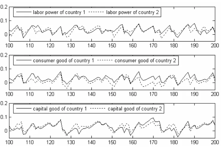
For concreteness, let’s give a numerical example of the growth model with m agents and n goods, which describes the dynamics of a simple two-country economy.

Suppose there are two countries, i.e. country 1 and country 2, and each country consists of 3 agents, i.e. a household producing labor power, a consumer good producer and a capital good producer. Suppose consumer good and capital good are internationally tradable and labor power is internationally non-tradable. That is, agents of one country can only purchase the labor power supplied by the household of that country. Since the labor power of country 1 and country 2 isn’t substitutable for each other and as a result may have different prices, they need to be treated as two kinds of goods. Hence there are 6 agents and 4 goods in the model now.

Let’s index goods as follows:

Good 1 Labor power of country 1; Good 2 Consumer good;

Good 3 Capital good;

Good 4 Labor power of country 2. And agents are indexed as follows:

Agent 1 Household of country 1;

Agent 2 Consumer good producer of country 1; Agent 3 Capital good producer of country 1; Agent 4 Capital good producer of country 2; Agent 5 Consumer good producer of country 2; Agent 6 Household of country 2.

For the sake of simplicity, suppose each agent has only one technology and the unique technology matrix pair ( ,A B) consists of two matrices as follows:

0.28 0.50 0.53 0 0 0

0.84 0 0 0 0 0.77

0 0.49 0.45 0.50 0.48 0

0 0 0 0.51 0.57 0.29

A

é ù

ê ú

ê ú

=

ê ú

ê ú

ë û

,

1 0 0 0 0 0

0 1 0 0 1 0

0 0.25 1 1 0.25 0

0 0 0 0 0 1

B

é ù

ê ú

ê ú

=

ê ú

ê ú

ë û

.

( ) ( ) ( 1)

( ) ( )

0.98

, for 1, 2,3, 4

0.98 0.98

t t

t i i

i t t

i i

p u

p i

p u

+ ₌ìï > ₌

í _£

ïî (7.1)

 

( 1) ( ) ( ) ( )

0.8

t t t t

S + =Bz + e u S- (7.2)

(

( 1) ( 1)

)

(

( 1) ( 1)

)

, , ,

t t t t

u + z + =Z A p + S + (7.3)

(7.1) stands for the price adjustment process, which means if a good nearly clears its price won’t change, otherwise its price will fall by 2 percent. Here Assumption 5.1 is relaxed, and all prices won’t change if and only if all goods nearly clear. If there are goods far from clearing, the prices of nearly clearing goods will rise relatively. Since only relative prices matters in the model, such adjustment method is reasonable.

(7.2) stands for the formation of supplies. Here we assume a simple inventory depreciation function Q(M)=0.8M .

(7.3) stands for the exchange process. Note that T

B A is indecomposable here, as a result

(t 1)T

S + A is indecomposable for all t=1, 2,××× ¥, if (0)

z _0 holds. We set initial values as (0)

p =e, (0)

z =e, (0)

u =e, and compute the model for 200 periods. Some numerical results are shown in Figure 1, 2 and 3.

Since only relative prices matters, the price vector ( )t

p can be normalized such that ( )

1 T t

e p = , and normalized prices are shown in Figure 1.

The production intensities indicated by ( )t

z are shown in Figure 2, and the growth rates of components of ( )t

z , i.e. the growth rates of production intensities of 6 agents, are shown in Figure 3. For the model (7.1)-(7.3), we can readily find its balanced growth paths with the maximal growth rate (i.e. with the minimal cost rate), in which the growth rate and cost rate equal 0.0492 and 0.9531 respectively, the normalized price vector is

*

[0.2646 0.2120 0.2772 0.2462]T

p = ,

and the normalized production intensity vector is

*

[0.2725 0.3669 0 0.2038 0 0.1568]T

z = .

Comparing such balanced growth paths with the definition of equilibrium paths, i.e. Definition 6.1, it’s clear that these paths in fact can be regarded as equilibrium paths of the model (7.1)-(7.3).

Observing those computation results of the numerical example and comparing them with *

p and

*

z , we find following facts.

First, after around period 30, the price of each good enters an interval respectively and then keeps fluctuating in the interval. Compared with *

p , it’s clear that each price is in fact fluctuating around its corresponding price in *

[image:18.595.100.476.97.248.2] [image:18.595.108.471.284.435.2]

Figure 1. Normalized prices of goods in period 1 to 200.

Figure 2. Production intensities in period 1 to 200.

[image:18.595.105.475.461.707.2]

Second, on average the production intensities of agent 3 and agent 5 grow more slowly than other agents. As a result, both the market share of agent 3 in the capital good market and the market share of agent 5 in the consumer good market are decreasing. Furthermore, when we compute 20,000 periods of the model (7.1)-(7.3) and normalize those production intensity vectors, we find that with time passing by, the normalized production intensities of agent 3 and agent 5 are approaching to zero and the normalized production intensities of other agents keep fluctuating around those corresponding components of z* respectively.

Third, by aggregating data of agents belonging to each country, we find that country 1 keeps importing the capital good and exporting the consumer good in all periods, and country 2 is quite the contrary. That is, there emerges international specialization in this example.

Fourth, the growth rates of production intensities of agents fluctuate quite synchronously, as shown in Figure 3. That is, there are business cycles in the two-country economy. Moreover, when we compute 20,000 periods of the model (7.1)-(7.3), we find that the fluctuations of prices and growth rates show no sign of abating.

8. Discussion

Here, we discuss some results of this paper and some open questions.

A. Equilibrium: In the equilibrium analysis of this paper the existence of equilibrium paths depends on the existence of optimal TMP, and for the sake of simplicity we suppose each agent possesses a finite number of technologies so that there are a finite number of TMPs, thus the existence of optimal TMP is guaranteed. However, optimal TMP may still exist when this assumption is relaxed. In fact, Proposition 3.4 implies that even if each agent can use its technologies in combination, there still exist optimal TMP and equilibrium paths. In such case the technology set of each agent is in essence a compact convex set with a finite number of extreme points. In the future work the assumption on technology sets need to be weakened further to allow for merely close convex technology sets. And the equilibrium analysis in the case of m agents and n

goods is also left to the future work.

B. Disequilibrium: Though this paper pays much attention to equilibrium analysis, the model (5.1)-(5.5) may play a better role in disequilibrium analysis. And Proposition 3.2 can be interpreted as a simple result in disequilibrium analysis. The proposition implies in any period of any path of the model (5.1)-(5.5) there is one agent whose minimal cost rate is no greater than *

l .

normalized price vector will keep fluctuating in a neighborhood of the normalized equilibrium price vector. Behaviors of the model in more complicated cases, e.g. each agent possesses a wide range of technologies, needs further studies. And numerical methods such as Monte Carlo simulation are likely to play an important role in the future disequilibrium analysis.

C. Changing Technology Sets: In this paper technology sets of agents are supposed to be exogenous and time-invariant. The assumption can be relaxed to allow that technology sets vary gradually as other variables changing, e.g. as output levels rising or time passing by. Such changing technology sets can be used to treat changing returns to scale, technology progress etc. And for this purpose an equation standing for the changing of technology sets need to be added to the grow model. So far as numerical methods are adopted, such dynamic technology sets won’t bring essential difficulties to the analysis of the model.

D. Multi-country Economic Analysis: As shown by the two-country example, the model in this paper treats a country merely as a set of agents. Thus for the model in this paper, describing and analyzing a k-country economy is essentially the same as describing and analyzing a national economy. And macroeconomic variables of each country can be obtained easily by aggregating variables of its agents. By running such model on computer, the propagation of effects of a single agent’s microeconomic change through a k-country economy can be traced and studied as if we were doing a laboratory experiment.

References

Bapat, R. B., D. D. Olesky, and P. van den Driessche (1995) Perron_–Frobenius Theory for a Generalized Eigenproblem, Linear and Multilinear Algebra, 40, 141_–152.

Debreu, G. and I. N. Herstein (1953) Nonnegative Square Matrices, Econometrica, 21, 597-607. Dempster, M. A. H., I. V. Evstigneev and M. I. Taksar (2006) Asset Pricing and Hedging in

Financial Markets with Transaction Costs: An Approach Based on the von Neumann_–Gale Model,

Annals of Finance, 2, 327_–355.

Dorfman, R., P. A. Samuelson and R. M. Solow (1958) Linear Programming and Economic Analysis. New York: McGraw-Hill.

Evstigneev, I. V. and K. R. Schenk-Hoppe (2007) Pure and Randomized Equilibria in the Stochastic von Neumann_–Gale Model, Journal of Mathematical Economics, 43, 871_–887.

Gale, D. (1956) The Closed Linear Model of Production, in Linear Inequalities and Related Systems,

Ed. By H. W. Kuhn and A. W. Tucker. Princeton, N.J.: Princeton University Press, 285-303. Gale, D. (1960) The Theory of Linear Economic Models. New York: McGraw-Hill.

Horn, R. A., and C. R. Johnson (1990) Matrix Analysis. Cambridge: Cambridge University Press. Kemeny, J. G., O. Morgenstern and G. L. Thompson. (1956) A Generalization of the von Neumann

Leontief, W. (1936) Quantitative Input-Output Relations in the Economic System of the United States, Review of Economics and Statistics, 18: 105-125.

Leontief, W. (1941) Structure of the American Economy, 1919-1929. Cambridge, Mass.: Harvard University Press.

Mangasarian, O. L. (1971) Perron-Frobenius Properties of Ax-λ_{Bx, Journal of Mathematical}

Analysis and Application, 36, 86–102.

McKenzie, L. W. (1963) Turnpike Theorems for a Generalized Leontief Model, Econometrica, 31, 165-180.

McKenzie, L. W. (1976) Turnpike Theory, Econometrica, 44, 841-865.

Mehrmann, V., R. Nabben and E. Virnik (2008) Generalisation of the Perron–Frobenius Theory to Matrix Pencils, Linear Algebra and its Applications, 428, 20–38.

Morishima, M. (1960) Economic Expansion and the Interest Rate in Generalized von Neumann Models, Econometrica, 28, 352-363.

Morishima, M. (1964) Equilibrium, Stability and Growth: A Multi-sectoral Analysis. New York: Oxford University Press.

von Neumann, J. (1945) A Model of General Economic Equilibrium, Review of Economic Studies, 13, 1–9.

Solow, R, and P. Samuelson (1953) Balanced Growth under Constant Returns to Scale,

Econometrica, 21, 412-424.