Burr Type XII Software Reliability Growth Model

Burr Type XII Software Reliability Growth Model

R. Satya Prasad,

Ph.D Associate Professor Department of CSE Acharya Nagarjuna

University Guntur, India

K.V. Murali Mohan

Associate Professor Department of ECE H.M. Institute of Tech. and

Science Hyderabad, India

G. Sridevi

Associate Professor Department of CSE Nimra Women’s College of

Engg Vijayawada, India

ABSTRACT

Software Reliability Growth model (SRGM) is a mathematical model of how the software reliability improves as faults are detected and repaired. The development of many SRGMs over the last several decades have resulted in the improvement of software facilitating many engineers and managers in tracking and measuring the growth of reliability. This paper proposes Burr type XII based Software Reliability growth model with time domain data. The unknown parameters of the model are estimated using the maximum likelihood (ML) estimation method. Reliability of a software system using Burr type XII distribution, which is based on Non-Homogenous Poisson process (NHPP), is presented through estimation procedures. The performance of the SRGM is judged by its ability to fit the software failure data. How good does a mathematical model fit to the data is also being calculated. To access the performance of the considered SRGM, we have carried out the parameter estimation on the real software failure datasets.

General Terms

Software failure data, Mean value function.

Keywords

Software Reliability, Burr type XII distribution, NHPP, ML Estimation

1.

INTRODUCTION

Software reliability is defined as the probability of failure free software operation for a specified period of time in a specified environment (Lyu, 1996) (Musa et al.. 1987).SRGM is a mathematical model of how the software reliability improves as faults are detected and required (Quadri and Ahmad, 2010). Among all SRGMs developed so far a large family of stochastic reliability models based on a Non-Homogeneous Poisson Process known as NHPP reliability model has been widely used. Software Reliability is the most dynamic quality characteristic which can measure and predict the operational quality of the software system during its intended life cycle. To identify and eliminate human errors in software development process and also to improve software reliability, the Statistical Process Control concepts and methods are the best choice. If the selected model does not fit the collected software testing data relatively well. We would expect a low prediction ability of this model and the decision makings based on the analysis of this model would be far from what is considered to be optimal decision (xie et al., 2001). This paper presents a method for model validation.

2. RELATED RESEARCH

This section presents the theory that underlies the proposed distributions and maximum likelihood estimation for complete data. If „t‟ is a continuous random variable

with pdf:

f t

( ; ,

 

_{1 2}

,...,



_k

)

. Where

 

₁

,

₂

,...,



_k are k unknown constant parameters which need to be estimated, and cdf:

F t

( )

. Where, the mathematical relationship between the pdf and cdf is given by:

( ( ))

( )

d F t

f t

dt



. Let „a‟ denote the expected number

of faults that would be detected given infinite testing time in case of finite failure NHPP models. Then, the mean value function of the finite failure NHPP models can be written as:

m t

( )



aF t

( )

. Where,

F t

( )

is a cumulative distributive function. The failure intensity function



( )

t

in case of the finite failure NHPP models is given by:

'

( )

t

aF t

( )





[8].

2.1 NHPP Model

There are numerous software reliability growth models available for use according to probabilistic assumptions. The Non Homogenous Poisson Process (NHPP) based software reliability growth models are proved to be quite successful in practical software reliability engineering [4]. Model parameters can be estimated by using maximum Likelihood Estimate (MLE). NHPP model formulation is described in the following lines.

A software system is subjected to failures at random times caused by errors present in the system. Let



N t t

( ),



0



be a counting process representing the cumulative number of failures by time „t‟, where t is the failure intensity function, which is proportional to the residual fault content.

Let

m t

( )

represent the expected number of software failures by time „s‟. The mean value function

m t

( )

is finite valued, non-decreasing, non-negative and bounded with the boundary conditions.

0,

0

( )

,

t

m t

a t





 

_{ }



Suppose

N t

( )

is known to have a Poisson probability mass function with parameters

m t

( )

i.e.,

𝑃 𝑁 𝑡 = 𝑛 =

𝑚 𝑡

𝑛

. 𝑒

−𝑚 𝑡

𝑛!

, 𝑛 = 0,1,2 …

∞

Then

N t

( )

is called an NHPP. Thus the stochastic behaviour of software failure phenomena can be described through the

N t

( )

process. Various time domain models have appeared in the literature that describes the stochastic failure process by an NHPP which differ in the mean value function

m t

( )

.

2.2. Proposed Model Description

In this paper, we propose to monitor software quality using SPC based on Burr Type XII distribution model. The Burr distribution has a flexible shape and controllable scale and location which makes it appealing to fit to data. It is frequently used to model insurance claim sizes [5]. The mean value function and intensity function of Burr Type XII NHPP model are as follows.

The Cumulative distributive function (CDF) is given by





1

0

( )

( )

1

1

c b

m t





t dt



a



_

 

t





_







(2.2.1)



a F t

( )

The Probability Density Function (PDF) of Burr XII distribution are given, respectively by





1

1

( )

( )

1

c

b c

cbt

t

a

a f t

t



 















_







Where t>0, a>0, b>0 and c>0 denote the expected number of faults that would be detached given infinite testing time in case of finite failure NHPP models. In order to have an assessment of the software reliability, a, b and c are unknown parameters and estimated by using Newton Raphson method. Expressions are now delivered for estimating „a‟, „b‟ and „c‟ for the Burr type XII model.



( )





( )



( )

!

n _{m t}

m t

e

p N t

n

n







lim



( )



.

!

a n

n

e

a

p N t

n

n









This is also a Poisson model with mean „a‟.

Let N (t) be the number of errors remaining in the system at time„t‟.

𝑁 𝑡 = 𝑁 ∞ − 𝑁 𝑡

𝐸 𝑁 𝑡 = 𝐸 𝑁 ∞ − 𝐸 𝑁 𝑡

 

a

m t

( )

 

a a



_

1 (1

 

t

c

)

b



_



a

(1



t

c

)

b

Let 𝑆𝑘 be the time between (𝑘 − 1)𝑡ℎ and 𝑘𝑡ℎ failure of

the software product. Let 𝑋𝑘 be the time up to the 𝑘𝑡ℎ

failure. Let us find out the probability that time between

(𝑘 − 1)𝑡ℎ _{and 𝑘}𝑡ℎ _{failures, i.e., 𝑆}

𝑘 exceeds a real number

„s‟ given that the total time up to the (𝑘 − 1)𝑡ℎ _{failure is}

equal to 𝑥. i.e., 𝑃 𝑆𝑘>_𝑋𝑠

𝑘−1= 𝑥

𝑅 𝑆𝑘/𝑋𝑘−1 𝑠/𝑥 = 𝑒− 𝑚 𝑥+𝑠 −𝑚(𝑠) (2.2.2)

This Expression is called Software Reliability.

3. ILLUSTRATING THE MLE

3.1. Parameter Estimation based on Time

Domain Data

In this section we develop expressions to estimate the parameters of the Burr type XII model based on time domain data. Parameter estimation is of primary importance in software reliability prediction.

A set of failure data is usually collected in one of two common ways, time domain data and time domain data. In this paper parameters are estimated from the time domain data.

The mean value function of Burr type XII model is given by





( )

1

1

c b

,

0

m t



a



_

 

t





_

t







(3.1.1)

We conduct an experiment and obtain N independent

observations

t t

₁

, ,...,

₂

t

_n. The likelihood function for time domain data [4] is given by

1

1 (1 ) 1

1

(1

)

.

c b b

N

a t

c c

i i

i

L

abct

t

e





 

  

  









1

(1

)

(

1) log

(

1) log(1

)

n

c b c

i i

i

LogL

a

a

t



Log a

Log b

Log c

c

t

b

t







  







_





 

 



_

(3.1.2)

i.e.,

Log L

0

a



_



(1

)

(1

)

1

c b c b

n

t

a

t



 





(3.1.3)

The parameter „b‟ is estimated by iterative Newton Raphson Method using

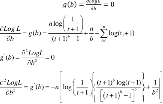
𝑏𝑛+1= 𝑏𝑛−_𝑔𝑔(𝑏)′_(𝑏) , Where 𝑔 𝑏 𝑎𝑛𝑑 𝑔′(𝑏) are expressed as follows.

𝑔 𝑏 =

𝜕𝐿𝑜𝑔𝐿_𝜕𝑏

= 0

1

1

log

1

( )

log(t

1)

(

1)

1

n i b

i

n

Log L

t

n

g b

b

t

b













_

_







_{ }

_









(3.1.4)

2 '

2

( )

LogL

0

g b

b













2

'

2

2 2

1

(

1) log(

1)

1

( )

log

1

₁

₁

b

b

LogL

t

t

g b

n

b

t

_t

b











_

_{ }















_

















_

_



_

_

_

_

_

_

_

_













(3.1.5)

The parameter „c‟ is estimated by iterative Newton Raphson Method using

𝑐𝑛+1= 𝑐𝑛 −_{𝑔′ 𝑐}𝑔 𝑐𝑛

𝑛

Where 𝑔 𝑐 𝑎𝑛𝑑 𝑔′ 𝑐 are expressed as follows.

𝑔 𝑐 =𝜕𝐿𝑜𝑔𝐿_𝜕𝑐 = 0

1 1

( )

log( )

2 log( )

log

(1

)

(1

)

c

n n

i

i

c c

i i i

t

LogL

n

n

g c

t

t

t

c

t

c



t





_

_



_{ }

_











(3.1.6)

𝑔′ 𝑐 =𝜕2_𝜕𝑐𝐿𝑜𝑔𝐿₂ = 0

2

'

2 2 2 2

1

log

1

( )

log

2 log .

log

(1

)

(1

)

c n

c

i i

c c

i i

Log L

nt

t

n

g c

t

t

t

t

c

t

c



t







_

_

_

_











_



_

(3.1.7)

4. DATA ANALYSIS

[image:3.595.80.355.193.369.2]

The set of software errors analyzed here is borrowed from software development project as published in Pham (2006) [8].

Table 1: Naval Tactical Data System Software Dataset

Failure Number

(n)

Time Between Failures (xk) days

Cumulative Time

(Sn)

1 9 9

2 12 21

3 11 32

4 4 36

5 7 43

6 2 45

7 5 50

8 8 58

9 5 63

10 7 70

11 1 71

12 6 77

13 1 78

14 9 87

15 4 91

16 1 92

18 3 98

19 6 104

20 1 105

21 11 116

22 33 149

23 7 156

24 91 247

25 2 249

26 1 250

Test Phase

27 87 337

28 47 384

29 12 396

30 9 405

31 135 540

User Phase

32 258 798

Test Phase

33 16 814

34 35 849

Solving equations by Newton Raphson Method for the NTDS test data, the iterative solutions for MLEs of a, b and c are

[image:4.595.74.297.69.418.2]

𝑎 = 26.105273 𝑏 = 0.998899 𝑐 = 0.998903

Table 2 : Parameters Estimated through MLE

Dataset

Number of samples

Estimated Parameters

a b c

NTDS 26 26.105273 0.998899 0.998903

Xie 30 30.040800 0.999825 0.999619

AT & T 22 22.032465 0.999859 0.999611

IBM 15 15.051045 0.999530 0.999196

SONATA 30 30.016391 0.999958 0.999920

Hence, we may accept these three values as MLSs of The estimator of the reliability function from the equation (2.2.2) at any time x beyond 250 hours is given by

𝑅 𝑆

𝑘

/𝑋

𝑘−1

𝑠/𝑥 = 𝑒

− 𝑚 𝑥+𝑠 −𝑚(𝑠)

[ (50 250) (250)] 7

/

6

(250 / 50)

m m

R s

x



e

  

[ (300) (250)]

0.98269972

m m

e

 





5. METHOD OF PERFORMANCE

ANALYSIS

[image:4.595.72.302.513.709.2]

The performance of SRGM is judged by its ability to fit the software failure data. The term goodness of fit denotes the question of “How good does a mathematical model fit to the data?”. In order to validate the model under study and to assess its performance, experiments on a set of actual software failure data have been performed. The considered model fits more to the dataset whose Log Likelihood is most negative. The application of the considered distribution function and its Log Likelihood on different datasets collected from real world failure data is given below.

Table 3 : Log Likelihood on different datasets

Data Set Log L (MLE) Reliability

(tn+x)

NTDS - 38.477204 0.98269972

Xie - 44.402007 0.99616300

AT & T - 18.949300 0.99573348

IBM - 27.365034 0.98841341

SONATA - 46.991596 0.99700207

6.

CONCLUSION

To validate the proposed approach, the parameter estimation is carried out on the data sets collected from (Xie et al., 2002; Pham, 2006; Ashoka, 2010).Out of the data sets that were collected, the model under consideration best fits the data of SONATA using MLE approach. Since, it is having the highest negative value for the log likelihood. The reliability of all the data sets are given in Table 3.The reliability of the model over SONATA data is high among the data sets which were considered.

7.

REFERENCES

[1] Kimura, M., Yamada, S., Osaki, S., 1995. ”Statistical Software reliability prediction and its applicability based on mean time between failures”. Mathematical and Computer Modelling Volume 22, Issues 10-12, Pages 149-155.

[2] Ashoka, M., (2010), “Sonata Software Limited” data set, Bangalore.

[3] Lyu, M.R., (1996), “Handbook of Software Reliability Engineering”, MCGraw-Hill, New York.

[4] Musa, J.D., Iannino, A., Okumoto, k., 1987. “Software Reliability: Measurement Prediction Application”. McGraw -Hill, New York.

[6] Pham. H., 2003. “Handbook of Reliability Engineering”, Springer.

[7] Pham. H., 2006. “System software reliability”, Springer.

[8] Swapna S. Gokhale and Kishore S.Trivedi, 1998. “Log-Logistic Software Reliability Growth Model”. The 3rd IEEE International Symposium on High-Assurance Systems Engineering. IEEE Computer

Society.

[9] Xie, M., Goh. T.N., Ranjan.P., (2002) “Some effective control chart procedures for reliability monitoring” – Reliability engineering and System Safety 77 143 -150 ̧ 2002.

[10]Satya Prasad, R., “Half logistic distribution for software reliability growth model”, Ph.D thesis, 2007.

[11]Goel, A.L., Okumoto, K., 1979. Time-dependent error detection rate model for software reliability and

other performance measures. IEEE Trans. Reliab. R-28, 206-211.

[12]Satya Prasad, R., Shaheen., Krishna Mohan, G., “Two step Approach for Software reliability: HLSRGM”, IJCTT-Volume 4 Issue 10-Oct 2013.

[13]Wood, A., (1996), “Software Reliability Growth models”, Tandem Computers, Technical report 96.1.

[14]Quadri, S.M.K and Ahmad, N., (2010), “Software Reliability Growth Modelling with new modified Weibull testing-effort and optimal release policy”, International Journal of Computer Applications, Vol.6, No.12.