
http://dx.doi.org/10.4236/jpee.2016.41001
How to cite this paper: Kramm, G., Sellhorst, G., Ross, H.K., Cooney, J., Dlugi, R. and Mölders, N. (2016) On the Maximum of Wind Power Efficiency. Journal of Power and Energy Engineering, 4, 1-39. http://dx.doi.org/10.4236/jpee.2016.41001
On the Maximum of Wind Power Efficiency
Gerhard Kramm1*, Gary Sellhorst2, Hannah K. Ross3, John Cooney4, Ralph Dlugi5,Nicole Mölders6
1Engineering Meteorology Consulting, Fairbanks, USA
2Geophysical Institute, University of Alaska Fairbanks, Fairbanks, USA
3Department of Mechanical Engineering, University of Washington, Seattle, USA 4Department of Atmospheric Sciences, Texas A & M University, College Station, USA 5Arbeitsgruppe Atmosphärische Prozesse (AGAP), Munich, Germany
6College of Natural Science and Mathematics and Geophysical Institute, University of Alaska Fairbanks, Fairbanks, USA
Received 7 October 2015; accepted 26 December 2015; published 29 December 2015
Copyright © 2016 by authors and Scientific Research Publishing Inc.
This work is licensed under the Creative Commons Attribution International License (CC BY).
http://creativecommons.org/licenses/by/4.0/
Abstract
In our paper we demonstrate that the filtration equation used by Gorban’ et al. for determining the maximum efficiency of plane propellers of about 30 percent for free fluids plays no role in de-scribing the flows in the atmospheric boundary layer (ABL) because the ABL is mainly governed by turbulent motions. We also demonstrate that the stream tube model customarily applied to derive the Rankine-Froude theorem must be corrected in the sense of Glauert to provide an appropriate value for the axial velocity at the rotor area. Including this correction leads to the Betz-Joukowsky limit, the maximum efficiency of 59.3 percent. Thus, Gorban’ et al.’s 30% value may be valid in water, but it has to be discarded for the atmosphere. We also show that Joukowsky’s constant cir-culation model leads to values of the maximum efficiency which are higher than the Betz-Jow- kowsky limit if the tip speed ratio is very low. Some of these values, however, have to be rejected for physical reasons. Based on Glauert’s optimum actuator disk, and the results of the blade-ele- ment analysis by Okulov and Sørensen we also illustrate that the maximum efficiency of propeller- type wind turbines depends on tip-speed ratio and the number of blades.
Keywords
Wind Power, Power Efficiency, General Momentum Theory, Axial Momentum Theory, Blade Element Analysis, Betz-Joukowsky Limit, Joukowsky’s Constant Circulation Model, Glauert’s Optimum Actuator Disk, Balance Equation for Momentum, Equation of Continuity, Balance Equation for Kinetic Energy, Reynolds’ Average, Hesselberg’s Average, Favre’s Average, Bernoulli’s Equation, Integral Equations
1. Introduction
In 2001, Gorban’ et al. [1] challenged the Betz limit (in our study called the Betz-Joukowsky limit [2]-[6] even though it has also been denoted as Lanchester-Betz-Joukowsky limit [2] [6]), i.e., the maximum power efficien-cy of 59.3 percent for a propeller-type turbine, where the power efficienefficien-cy is generally defined by
P
P C
P∞
= . (1.1)
Here, P is the extracted (or consumed) power, and P∞ is the power carried by the flow through the projection of the turbine section region onto the plane perpendicular to it. Gorban’ et al.[1] argued that the maximum effi-ciency of the plane propeller is about 30 percent for free fluids. Meanwhile, their paper has been cited numerous times in conference papers (e.g., [7] [8]), but recently van Kuik et al.[9] rejected their method and pointed out that the main problem of Gorban’ et al. “is their lack of comprehension of the working principles how the tur-bine operates”. Since this argument is very harsh, it is indispensable to show that the result of Gorban’ et al. is based on an equation that may be acceptable for water fluids of low flow velocity, but that is indeed not very suitable for flows as they are typical in the atmospheric boundary layer (ABL, the lowest layer of the tropos-phere, with a thickness of the order of h=10 m3 ), especially at heights between 30 mto 150 m above the Earth’s surface.
According to Gorban’ et al. [1], the filtration equation,
p r
−∇ = v, (1.2) holds in an open domain Vc (denoted by [1] as Ω) with a smooth or piecewise smooth boundary together with
the equation of continuity, ∇ ⋅ =v 0 (only valid for an incompressible stationary flow), where p and v denote the pressure and the velocity of the flow, respectively. The shape of Vcis considered as a semi-penetrable
ob-stacle for the stream with a resistance density r inside. Let Ac the cross section of Vc perpendicular to the flow
axis. The power carried by the flow through Ac is then given by 3
1
2 c
P∞ = ρA v∞. (1.3) Following these authors, v∞ is the velocity of a uniform laminar current. Gorban’ et al.[1] argued that the power, P, consumed by the turbine is given by
( )
2 21
d d d
c c c
V V V
P p V p V r V
r
=
∫
v⋅∇ =∫
∇ =∫
v , (1.4)where the filtration Equation (1.2) has been inserted. In accord with Equation (1.1), they obtained
3
d
1 2
c
V P
c
p V P
C
P∞ ρA v
∞
⋅∇ = =
∫
v
. (1.5)
Gorban’ et al. [1] claimed:
“The efficiency coefficient can be maximized by optimizing the resistance density. The optimal ratio between the streamlining current and the current passing through the turbines can also be obtained from this model. This parameter can be measured experimentally to determine how close a real turbine is to the theoretically optimal one.”
Obviously, the maximum of the efficiency coefficient deduced by Gorban’ et al.[1] depends on the filtration equation. This equation, however, plays no role in the description of ABL flows. In addition, the ABL is mainly governed by turbulent motions. If we assume, for instance, a wind speed of v =7.5 m s⋅ −1 at a hub height of
80 m
z= and a kinematic viscosity of ν =1.5 10× −5 m2⋅s−1
we will obtain a Reynolds number of about
1
7
5 2 1
7.5 m s 80 m 4 10 1.5 10 m s
z Re
ν
−
− −
⋅ ×
= = = ×
× ⋅
v
flow occurs.
In the following section, we will present the governing equations for macroscopic and turbulent systems rele-vant for wind power studies: (a) the local balance equations for momentum (also called the Navier-Stokes equa-tion), (b) total mass (also called the equation of continuity), and (c) kinetic energy. It is shown that the Bernoulli equation for an incompressible flow can simply be derived from the local balance equation of kinetic energy. Furthermore, we will derive the simplified integral balance equations recently used by Sørensen [6] in his re-view on the aerodynamic aspects of wind energy conversion to incorporate his results in our discussion. Addi-tionally, we will demonstrate that Equation (1.4) derived by Gorban’ et al. [1] is incomplete for the ABL so that their maximum efficiency calculation for plane propellers of about 30 percent for free fluids has to be discarded, as suggested by van Kuik et al. [9]. This means that the filtration Equation (1.2) is meritless if the maximum ef-ficiency of wind power has to be determined. In Section 3, we will discuss the main characteristics of propel-ler-type wind turbines. Our discussion will include the basics of the axial momentum theory, Joukowsky’s con-stant circulation model, Glauert’s infinite-bladed actuator disk model, and finite-bladed rotor models. We will show that the Betz-Joukowsky limit is, indeed, the maximum of the wind power efficiency, even though some results of Joukowsky’s constant circulation model might exceed it because of physically inadequate conditions. Glauert’s [10] optimum actuator disk and finite-bladed rotors [6] [11] [12] tend to this maximum, if the tip- speed ratio, λ, increases.
2. Theoretical Background
2.1. The Governing Equations for the Macroscopic System
In order to outline the generation of electricity by extracting kinetic energy from the wind field we consider the local balance equations for momentum (i.e., Newton’s 2nd axiom), Equation (2.1), and total mass, Equation (2.2), for a macroscopic system given by (e.g., [13]-[16]):
( )
(
)
(
)
2 p
t ρ
ρ ρ ϕ ρ
∂
+ ∇ ⋅ + + = − ∇ − ×
∂ Ω
v
vv E J v (2.1)
and
( )
0t
ρ ρ
∂ + ∇ ⋅ =
∂ v . (2.2)
Here, ρ is the air density, t is time, v is the velocity of the flow, J is the Stokes stress tensor given by
( )
(
T)
2(
)
3
d
ρν µ ρν
= ∇ + ∇ + − ∇ ⋅
J v v v E. (2.3)
where µd is the bulk viscosity (near zero for most gases), E is the identity tensor, ϕ is the gravity
poten-tial, and Ω is the angular velocity of the Earth. Both J and E are symmetric second-rank tensors. Fur-thermore, the 1st term of the left-hand side of Equation (2.1) describes the local temporal change of momentum, and the 2nd term represents the exchange of momentum between the system under study and its surroundings, where p E+J exerts on the boundary of this system. The 1st term on the right-hand side of this equation represents the gravity force, and the 2nd one the Coriolis force. Equation (2.2) is the equation of continuity. In addition, local balance equations for various energy forms (i.e., internal energy, kinetic energy, potential energy, and total energy), various water phases (i.e., water vapor, liquid water, and ice), and gaseous and particulate at-mospheric trace constituents exist. All these local balance equations can be derived from integral balance equa-tions (e.g., [13] [14]). Since D
( )
ρv Dt= ∂( )
ρv ∂ + ∇ ⋅t(
ρvv)
=ρd dv t and ∇ ⋅( )
pE = ∇p, Equation (2.1) is often written as (e.g., [17]-[19])(
)
1
2 p
t ρ ρ ϕ
∂ + ⋅∇ + ∇ ⋅ = −∇ − ∇ − × ∂
v
v v J Ω v , (2.4)
(
)
2
2
⋅ ∇ = ∇ − × ∇×
v
v v v v , (2.5)
Equation (2.4) may be written as
(
)
2
1 1
2
2 p
t ρ ρ ϕ
∂ + ∇ − × ∇× + = − ∇ ⋅ − ∇ − ∇
∂ Ω
v v
v v J . (2.6)
The curl of Equation (2.6) leads to the prognostic equation for the vorticity
(
)
2(
(
)
)
1 1
2
2 p
t ρ ρ ϕ
∂ ∇× + ∇×∇ − ∇× × ∇× + = − ∇× ∇ ⋅ − ∇× ∇ − ∇×∇
∂ Ω
v
v v v J , (2.7)
As the curl of the gradient of a scalar field is equal to zero, Equation (2.7) can be written as
(
)
(
(
)
)
1 12 p
t ρ ρ
∂ ∇ × + ∇ × ∇ × + × = −∇ × ∇ ⋅ − ∇ × ∇
∂ v v Ω v J . (2.8)
This equation plays an important role in the description of rotational flows as occurred in the wake of the wind turbine. If the friction effect is negligible and the density is considered as spatially constant like in case of an incompressible fluid we will obtain
(
)
(
(
2)
)
0t
∂ ∇ × + ∇ × ∇ × + × =
∂ v v Ω v . (2.9)
To deduce the local balance equation for the kinetic energy of the flow, Equation (2.1) has to be scalarly mul-tiplied by the velocity vector v. Using the identities
(
p)
{
p}
:(
p)
{
p} (
p)
:⋅∇ ⋅ + = ∇ ⋅ + ⋅ − ∇ + = ∇ ⋅ + ⋅ − + ∇
v E J v v J v E J v v J E J v (2.10)
and
:
pE ∇ = ∇ ⋅v p v (2.11) leads to
2 2
:
2 2 p p
t ρ ρ ρ ϕ
∂ + ∇ ⋅ + + ⋅ = − ⋅ ∇ + ∇ ⋅ + ∇
∂
v v
v v J v v J v. (2.12)
The colon expresses the double-scalar product (also called the double dot product) of the tensor algebra. Fur-thermore, v⋅
(
Ω×v)
= ⋅ ×Ω(
v v)
=0. The 1st term of the left-hand-side of Equation (2.12) describes the local temporal change of kinetic energy, and the 2nd term is the energy exchange of the system with its surroundings which is performed by the surrounding air on the boundary of the system. The 1st term of the right-hand-side represents the conversion of potential energy into kinetic energy and vice versa, the 2nd term describes the re-versible work rate of expansion, ∇ ⋅ >v 0, or contraction, ∇ ⋅ <v 0, and the 3rd term represents the irreversible work rate owing to viscous friction. This term represents the dissipation of kinetic energy into the reservoir of heat. The term of our primary interest reads2
2
kin=ρ
v
S v. (2.13) It describes the transport of kinetic energy by the flow, and it may be called the kinetic energy stream density, but it is also denoted as wind power density. Inserting the definition of the total pressure,
2
2
H= +p ρv , (2.14) into Equation (2.12) yields
(
)
:H p
H p
t t ρ ϕ
∂ ∂
+ ∇ ⋅ + ⋅ = − ⋅ ∇ + ∇ ⋅ + ∇
2.2. The Governing Equations for the Turbulent System
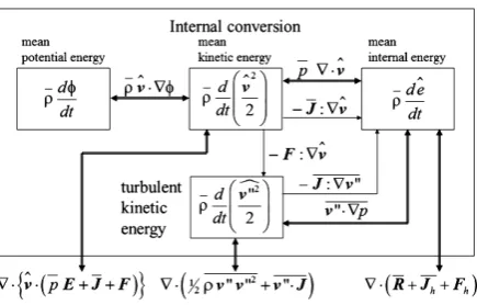
Since the ABL is mainly governed by turbulent motion, the use of the macroscopic balance Equations (2.1), (2.2), and (2.12) is rather impracticable. Therefore, these balance equations are customarily averaged in the sense of Reynolds [20]. However, conventional Reynolds averaging will lead to various short-comings in the set of governing equations for turbulent atmospheric flow, even if these averaging techniques can be performed ac-curately [22]. If we ignore, for instance, density fluctuation terms, the possibility to describe physical processes as a whole will clearly be restricted (see [23] [24]). The key questions that still remain are (a) how to average the governing macroscopic equations in the case of turbulent atmospheric flows and (b) what are the consequences of such an averaging, not only for momentum and total mass, but also for various energy forms like kinetic en-ergy, potential enen-ergy, internal enen-ergy, and total enen-ergy, consisting of the sum of these three energy forms. In the terrestrial atmosphere, the total energy is conserved. As sketched inFigure 1 for a turbulent system (Hes-selberg fluid), there are various ways of energy conversion.
As argued by various authors [22]-[34], the density-weighted averaging procedure suggested by Hesselberg [35] is very appropriate to formulate the balance equation for turbulent systems. It is given by
ρχ
χ ρ
= , (2.16)
where χ is a field quantity like the wind vector, v, the specific internal energy, e, and the specific enthalpy, h. Furthermore, the overbar () characterizes the conventional Reynolds mean. Whereas the hat () denotes the density-weighted average according to Hesselberg, and the double prime (") marks the departure from that. It is obvious that ρ χ"=ρχ"=0. The Hesselberg mean of the wind vector, for instance, is given by v=ρ ρv . Note that intensive quantities like the pressure, p, and the density, ρ, of air are averaged in the sense of Rey-nolds. Arithmetic rules can be found, for instance, in [25]-[27] [29] [31]. As pointed out by Kramm and Meixner [22] and Lumley and Yaglom [36], Hesselberg’s average is sometimes misnamed the Favre average.
[image:5.595.206.424.432.571.2]In comparison with that of Reynolds, Hesselberg’s averaging calculus leads to several prominent advantages [22] [25]-[27] [29]-[31] [35]: (a) The equation of continuity,
Figure 1. Schematic representation of the energy conversion
within a turbulent system (Hesselberg fluid) and the exchange of energy with its surroundings which is performed by the surrounding air on the boundary of the system. As illustrated in this sketch, there is no direct conversion of mean internal energy into mean potential energy and vice versa. Note that
S IR
= +
R R R is the total irradiance, where RS is solar
irradi-ance and RIR is the infrared irradiance. Furthermore, Jh and h=ρ ′′h
( )
0 tρ ρ
∂
+ ∇ ⋅ =
∂ v , (2.17)
keeps its form, and (b) the mean value of kinetic energy can exactly be split into the kinetic energy of the mean motion and mean value of the kinetic energy of the eddying motion, according to
(
)
2 2
2 2 2
1 1 1
" "
2 2 2 2
ρ
ρv = ρv + ρv = v +v . (2.18) This advantage is especially important in the theoretical description of the extraction of the kinetic energy from the wind field for generating electricity. The use of density-weighted averages is the common way to de-fine averages in studies of highly compressible turbulent flows (see also [29] [32]), probably the most natural way to define averages. The kinetic energy of the mean motion is usually abbreviated by MKE, and the kinetic energy of the eddying motion is usually called the turbulent kinetic energy abbreviated by TKE.
Hesselberg’s average procedure will be applied within the framework of this contribution. It can be related to that of Reynolds by (e.g., [22] [26] [30] [31] [37])
' ' ' '
1
ρ χ ρ χ
χ χ χ
ρ ρ χ
= + = +
. (2.19) Here, the prime (') denotes the deviation from the Reynolds mean. Obviously, the different means, χ and χ, are nearly equal if ρ χ' '
{ }
ρ χ 1 as used, for instance, in case of the Boussinesq approximation. In case of a nearly incompressible fluid, the distinction between v and v is not necessary because the condition{ }
' ' 1
ρ v ρ v is clearly fulfilled. However, to avoid any kind of confusion, we keep our notation.
In the averaged form, the local balance equation for momentum of the turbulent atmosphere reads (e.g., [22] [25]-[27] [29] [35] [38])
( )
(
)
(
)
2 p
t ρ
ρ ρ ϕ ρ
∂
+ ∇ ⋅ + + + = − ∇ − ×
∂ Ω
v
vv E J F v , (2.20)
where F =ρv v" " is the Reynolds stress tensor. It results from averaging the term ρvv in Equation (2.1) leading to ρvv=ρvv +ρv v" ". Similar local balance equations can be derived for various energy forms (i.e., internal energy, kinetic energy, potential energy, and total energy), various water phases (i.e., water vapor, liquid water, and ice), and gaseous and particulate atmospheric trace constituents [22] [25]-[31] [38] [39].
Averaging Equation (2.12) provides the corresponding local balance equation for the kinetic energy
(
2)
(
2 )
(
)
2 2 1 2
" " " " "
2 2 2
" : : "
p t
p p
ρ ρ ρ
ρ ϕ
∂ + + ∇ ⋅ + + + ⋅ + + + ⋅
∂
= − ⋅∇ − ⋅ ∇ + ∇ ⋅ + ∇ + ∇
v v v v v v J F v v v J
v v v J v J v
(2.21)
Obviously, the local derivative with respect to time not only contains the MKE, but also the TKE as outlined by Equation (2.18). Assuming, for instance, steady-state condition leads to
(
2)
(
2 )
2 2
" 0 " const.
2 2
t
ρ ρ
∂ + = ⇒ + =
∂
v v v v (2.22)
great intensity of rotation and is characteristic for all turbulent flows. Except for the immediate vicinity of rigid walls, turbulent dissipation exceeds direct dissipation by several orders of magnitude depending on the Reynolds number (e.g., [18] [22]). Furthermore, the mean kinetic energy stream density reads
(
2)
2 1 2
" " "
2 2
kin
ρ ρ
= + +
S v v v v v . (2.23) This equation describes the transfer of MKE and TKE by the mean wind field and the transfer of TKE by the eddying wind field. Ignoring the turbulent effects yields
2
1 2
kin= ρ
S v v , (2.24) i.e., Skin is approximated by the MKE stream density. The magnitude of Skin is given by
2 3
1 1
2 2
kin = ρ = ρv
S v v , (2.25) where v =v. Apparently, this quantity expresses that the wind power density is proportional to the cube of the wind speed. The rotor of a wind turbine causes a divergence effect expressed by ∇ ⋅Skin ≠0.
Unfortunately, there is a notable inconsistency regarding the role of the turbulence intensity. According to de Vries [40], for instance, this quantity is Tiu =σu u, where σu is the standard deviation of the horizontal wind
speed and 2 2
"
u u
σ = is the corresponding variance. If we assume that only a horizontal component of the mean wind field exists, for the purpose of convenience, in the direction of the x-axis of a Cartesian coordinate frame, Equation (2.23) would provide
2 2
3
2 3
" " " 1 2 kin x u u u u ρ ρ ρ = + + v v
S (2.26)
or 2 2 3 3 2 3
" " "
1 u u u u u ρ ρ = + + v v
, (2.27)
i.e. we have still to consider the fluctuations of all components in this coordinate frame. On the other hand, de Vries [40] argued that the instantaneous value is given by u= +u u", and, hence, u3=
(
u+u")
3, i.e.,
(
)
3 3 2 3 " 3 " 3 "2 "3
u = u+u =u + u u + uu +u . (2.28) Since u" 0= , we have
2 3 3 3 2 3 "
1 3 u u
u u u u σ = + +
. (2.29)
The term 3 3
"
u u is only equal to zero when the probability distribution of u is symmetrical. Nevertheless, for estimating the effect owing to turbulence this term is ignored which leads to
3
(
)
3 2
1 3 u
u =u + Ti . (2.30) Ignoring the similar term in Equation (2.27) yields
2 2 2
3 3
2 2 2
1 u v w
u u
u u u
σ σ σ
= + + +
where 2 2
"
v v
σ = and 2 2
"
w w
σ = are the variances with respect to the y- and z-axis of a Cartesian coordinate frame. Thus, only in case of σu2 =σv2 =σw2 Equations (2.30) and (2.31) become identical, but such an equality
does not generally exist.Figure 2 shows that the mean and the median of the turbulence intensity depending at the height of 90 m [41]. The observations were performed at the offshore measurement platform FINO1 which is located 45 km north of the island of Borkum in the German Bight. For wind speeds ranging from 3 m s⋅ −1 to
1
25 m s⋅ − the mean and the median of the turbulence intensity are smaller than 0.1. This means that according to Equation (2.30), the effects of the turbulence intensity are smaller than 3 percent. As reported by Türk and Emeis [41], the same is true for this wind speed range at the 30 m height. The effect by turbulence may become more influential in case of aerodynamically rougher landscapes covered, for instance, with vegetation. In case of wind farms the effect by turbulence may considerably increase inside the array of wind turbines [42] [43].
To obtain the local balance equation of MKE, Equation (2.20) has to be scalarly multiplied by v leading to
(
)
(
)
2 2
:
2 2 p p
t ρ ρ ρ ϕ
∂ + ∇ ⋅ + + ⋅ + = − ⋅ ∇ + ∇ ⋅ + + ∇
∂
v v
v v J F v v J F v
(2.32)
or
(
)
{
}
(
)
:H p
H p
t t ρ ϕ
∂ ∂
+ ∇ ⋅ + ⋅ + = − ⋅ ∇ + ∇ ⋅ + + ∇
∂ v v J F ∂ v v J F v (2.33)
with
2
2
H =ρv + p. (2.34) The quantity H may be considered as the mean total pressure. Subtracting Equation (2.32) from Equation (2.21) yields
2 2 1 2
" " " " " " : " :
2 2 2 p
t
ρ ρ ρ
∂ + ∇ ⋅ + + ⋅ = − ⋅∇ + ∇ − ∇
∂
v v v v v v J v J v F v (2.35)
or
2 2 1 2
(
)
" " " " " : " : 1
2 2 2 Sf
t
ρ ρ ρ
∂ + ∇ ⋅ + + ⋅ = ∇ − ∇ −
[image:8.595.150.469.398.680.2]∂ v vv v v v J J v F v , (2.36)
Figure 2. Turbulence intensity depending on wind speed at 90 m height for
the period September 2003-August 2007 (taken from Türk and Emeis, [41]). The observations were performed at the offshore measurement platform FINO1
where
" ˆ :
f
p
S = ⋅ ∇
− ∇
v
F v (2.37) is a non-dimensional parameter characterizing the thermal stability of a turbulent flow. This stability parameter expresses the relative importance of the two TKE-terms. It may be interpreted as a generalized Richardson number. The difference between the well-known flux-Richardson number and the generalized Richardson num-ber results from the parameterization of v"⋅ ∇p [22] [27]. Besides the vertical effects also horizontal effects have to be regarded under certain circumstances. In case of Sf > ⇔0 v"⋅ ∇ >p 0, mechanically produced TKE is mainly consumed by Archimedean effects. Consequently, there exists a critical Sf-value given by
, 1
f cr
S = . It characterizes that the mechanical gain of TKE is equal to the thermal loss of TKE, i.e., the term
(
)
:∇ 1−Sf
F v becomes equal to zero, and the net production rate of TKE vanishes. As the turbulent dissipa-tion still acts as a sink of TKE, the turbulent flow will become more and more viscous (laminar). In case of
0 " 0
f
S < ⇔v ⋅ ∇ <p , TKE is generated mechanically and thermally. If the mechanically generated TKE is much smaller than the thermal gain of TKE, and, hence, negligible, free convective conditions, Sf ≤Sf fc, , will occur. In the remaining range, forced convective conditions may prevail, Sf fc, <Sf <0. Thermally neutral stratification is characterized by Sf =0. The 2nd-order balance equation (2.35) is the only balance equation that additionally arises from averaging a macroscopic balance equation (e.g., [18] [23]). In meteorological models, the balance equation of TKE (2.35) serves to derive the eddy diffusivities for momentum and—via the turbulent Prandtl number and the species-dependent turbulent Schmidt numbers—the eddy diffusivities for sensible heat, and water vapor. This method of parameterization is known as one-and-a-half-order closure (e.g. [22] [44] [45]). In the mesoscale model of the National Centers for Environmental Prediction (NCEP) and the Weather Research and Forecasting (WRF) model, it is realized with respect to the level 2.5 of Mellor and Yamada [46]-[48].
The local balance equation for the mean total energy 1
(
2 2)
" 2
tot
e = + +e φ v +v can be deduced fromFigure 1 leading to
( )
{
(
)
}
1 2" " " 0 2
tot
h h tot
e
e p
t
ρ
ρ ρ
∂
+ ∇ ⋅ + + + ⋅ + + + + + ⋅ =
∂ R J F v E J F v v v J . (2.38)
This equation demonstrates that no production or destruction of mean total energy within any given fixed volume exists (e.g., [22] [26] [27] [29]). Obviously, contributions of energy of different orders of magnitude are summed, where only a very small fraction of the total potential energy (or total internal energy), e+φ, is available for conversion into kinetic energy (e.g., [22] [49]-[52]).
From the perspective of the generation of electricity by extracting kinetic energy from the wind field, Equa-tions (2.17), (2.20), and (2.32) play the dominant role. To obtain a tractable set of equaEqua-tions, effects caused by molecular and turbulent friction, J+F, v⋅
(
J+F)
, and(
J+F)
:∇v, are usually ignored. In addition, in-compressibility (∇ ⋅ =v 0) and steady state (∂( )
∂ =t 0) conditions are presupposed. In doing so, the set of approximated equations reads( )
ρ 0∇ ⋅ v = , (2.39)
(
ρ p)
ρ ϕ 2ρ(
)
∇ ⋅ vv + E = − ∇ − Ω×v , (2.40) and
2
2 p
ρ ρ ϕ
∇ ⋅ + = − ⋅ ∇
v
v v . (2.41)
2.3. The Bernoulli Equation
2 2
0
2 2
p ρ ρ ϕ p ρ ρϕ
= ⋅ ∇ + + ⋅ ∇ = ⋅ ∇ + +
v v
v v v . (2.42)
Based on this condition, Bernoulli’s equation, which plays an important role in describing the conversion of wind energy, can simply be derived by considering this condition along a streamline. In accord with the natural coordinate frame for streamlines, the Nabla operator reads
( )
s( )
s( )
s( )
s s
s n b
∂ ∂ ∂
∇ = + +
∂ ∂ ∂
t n b
. (2.43)
Here, we consider a natural coordinate frame with the unit vectors ts, ns , and bs that form a right-
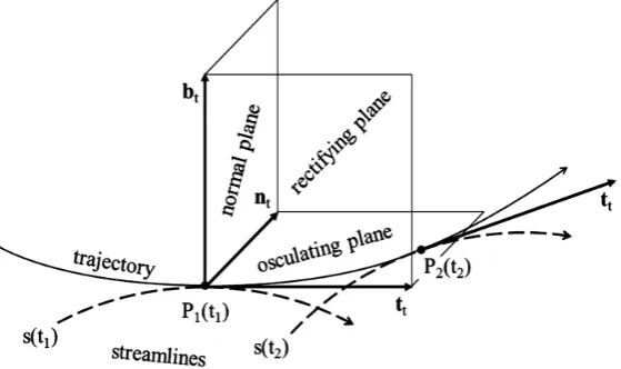
handed rectangular coordinate system at any given point of a curve in space (moving trihedron) like a trajectory or a streamline (see Figure 3), where the subscript s characterizes the streamline-related quantities. The velocity vector at a given point along the streamline is given by v=Vts =Vtt, where V is its magnitude, ts is the unit
tangent of the streamline, and tt is the unit tangent of the corresponding trajectory. The unit vectors ns and s
b are the principal normal and the binormal, respectively (e.g., [53] [54]). The different meaning of trajectories and streamlines is explained in theAppendix A.
With respect to Equation (2.43), the condition (2.42) results in
2 2
0
2 2
s s
V p V p
s ρ ρϕ s ρ ρϕ
∂ ∂
= ⋅ + + = + +
∂ ∂
v v
t t . (2.44)
This means that for any value of V ≠0, the condition
2
const. 2
[image:10.595.176.456.452.618.2]p+ρv +ρϕ= (2.45) is fulfilled along a streamline. Equation (2.45) is Bernoulli’s equation (e.g., [14] [15] [17] [55] [56]). Even though air density is considered as spatially constant, Bernoulli’s equation can often be applied to atmospheric flows. If the streamlines are mainly horizontally oriented and the variation of the gravity potential with height is small like in case of the swept area of a wind turbine, the variation of the gravity effect may be considered as negligible
Figure 3. Chronologically ordered streamlines (dashed lines) enveloped by a
trajectory (solid line). The trihedron at any point of the trajectory is given by the unit tangent, tt, the principal normal, nt, and the binormal, bt. The
−
t t
t n plane is called the osculating plane, the tt−bt plane is the rectifying
plane, and the nt−bt plane is the normal plane (e.g., [53] [54]). The
corre-sponding unit vectors of a streamline are ts, ns, and bs, where at a given
so that Equation (2.45) results in (e.g., [21] [56])
2
const. 2
H = +p ρv = (2.46) This approximation of Bernoulli’s equation customarily serves as the foundation of, and is used to derive the Rankine-Froude theorem.
2.4. The Integral Equations
The integration of Equations (2.39) to (2.41) over a time-independent control volume, encompassing the rotor of the wind turbine, yields [6] [56]
( )
d 0C
V
V ρ
∇ ⋅ =
∫
v , (2.47)(
)
d(
2(
)
)
dC C
V V
p V V
ρ ρ ϕ ρ
∇ ⋅ + = − ∇ + ×
∫
vv E∫
Ω v , (2.48)and
(
)
2
d d
2
C C
V V
p V V
ρ ρ ϕ
∇ ⋅ + = − ⋅ ∇
∫
v v∫
v . (2.49)In accord with Gauss’ integral theorem, Equation (2.47) and the left-hand side of Equation (2.48) can be writ-ten as
( )
( )
d d 0
C C
V A V
V A
ρ ρ
∇ ⋅ = ⋅ =
∫
v∫
v n (2.50)and
(
)
(
)
( )
d d
C C
V A V
p V p A
ρ ρ
∇ ⋅ + = + ⋅ =
∫
vv E∫
vv E n T, (2.51)where T is the thrust. Since ρvv is a second-rank tensor, it is advantageous to scalarly multiply Equation (2.48) by the unit vector ex from the left to get the more tractable equation
( ) ( )
(
(
)
)
d d 2 d
C C C
x x x x x
A V A V V
u A p A T V
ρ ⋅ + ⋅ = = − ρ ⋅ ∇ +ϕ ρ ⋅ ×
∫
v n∫
e n∫
e e Ω v . (2.52)Here, Tx =ex⋅T is the axial force acting on the rotor (e.g., [6]). If we assume that the axial direction
coin-cides with any horizontal direction, the term ex ⋅ ∇
ϕ
will be nearly equal to zero. Since the Coriolisaccelera-tion is given by 2Ω× = Ωv 2
(
wcosφ−vsinφ)
i+2uΩsinφj−2uΩcosφk, where φ is the latitude, and u, v, and w are the components of the mean wind vector in west-east direction (characterized by the unit vector i), south-north direction (characterized by the unit vector j), and the vertical direction (characterized by the unit vector k), respectively; the term 2ex⋅(
Ω×v)
= Ω2(
wcosφ−vsinφ)
ex⋅ +i usinφex⋅ j is very small for any wind speed smaller than the cut-out wind speed because Ω =7.27 10× −5rad s⋅ −1. Thus, this term is negligible, and Equation (2.52) may be approximated by
( ) ( )
d d
C C
x x x
A V A V
u A p A T
ρ ⋅ + ⋅ =
∫
v n∫
e n . (2.53)The second term of the left-hand side of this equation is usually ignored in the blade element momentum (BEM) theory. However, this term is not zero [6] [10] [57].
drical polar coordinates, respectively; and ex, er, and eθ are the corresponding unit vectors pointing in axial,
radial, and azimuthal direction. The azimuthal velocity component acting on the rotor at a certain radius r causes a torque given by
( )
d
C
A V
rvθ A Q
ρ ⋅ =
∫
v n . (2.54)In accord with Gauss’ integral theorem, the left-hand side of Equation (2.49)reads
( )
2 2
d d
2 2
C C
V A V
p V p A P
ρ ρ
∇ ⋅ + = + ⋅ =
∫
v v∫
v v n . (2.55)This term represents the power extracted by the rotor of the wind turbine. In case of a quasi-horizontal flow, the right-hand side of Equation (2.49) can be neglected because ∇ϕ is quasi-perpendicular to v. The effect of the gravity potential was already considered as negligible in Bernoulli’s Equation (2.45). The integral relation (2.55) underlines the importance of Bernoulli’s equation in wind power studies.
Rearranging the left-hand side of Equation (2.49) yields
( )
2 2
d d d
2 2
C C C
V V V
P ρ p V ρ V p V
= ∇ ⋅ + = ∇ ⋅ + ∇ ⋅
∫
v v∫
v v∫
v . (2.56)Because of ∇ ⋅ =v 0, the divergence term ∇ ⋅
( )
pv can be expressed by ∇ ⋅( )
pv = ⋅ ∇v p leading to2 2
d d d
2 2
C C C
V V V
P ρ p V ρ V p V
= ∇ ⋅ + = ∇ ⋅ + ⋅ ∇
∫
v v∫
v v∫
v . (2.57)Obviously, the first term on the right-hand side of this equation is missing in that of Gorban’ et al. [1], re-peated here by Equation (1.4). This means that the filtration Equation (1.2) that leads to Equation (1.4) is merit-less in determining the maximum efficiency of propeller-type wind turbines. Thus, the argument of van Kuik et al.[9] seems to be justified by Equation (2.57).
3. Wind Turbine Characteristics
3.1. The Axial Momentum Theory
3.1.1. The Rankine-Froude Theorem
In the following, we assume a pure axial flow (one-dimensional problem), i.e., the undisturbed wind speed far upstream of the wind turbine, v∞ , the wind speed at the rotor area, vR , and the undisturbed wind speed far
downstream of the wind turbine, vw , have the same direction so that we may consider only the magnitude of
these wind vectors expressed by v∞ , vR, and vw, respectively. Doing so agrees with the so-called stream-tube
model sketched in Figure 4, in which an “actuator disk” is representing the axial load on a rotor (e.g., [58]). This axial momentum theory was developed by Rankine [59], W. Froude [60], and R.E. Froude [61].
To derive the Rankine-Froude theorem we consider the variation of wind speed and pressure by approaching and leaving the rotor area as sketched in Figure 4, part A. In accord with Bernoulli’s equation in its approx-imated form (see Equation (2.46)), the former can be expressed by
2 2
2 2
R R
v v
H∞ = p∞ +ρ ∞ = p +ρ . (3.1) Whereas the latter is given by
2 2
2 2
w R
w R w
v v
(a) (b)
Figure 4. (a) Sketch of the stream-tube model; (b) Wind speed and pressure variations by approaching and leaving the rotor
area (with respect to Betz [58]). The stream-tube model is based on the equation of continuity expressed by Equation (3.7), where the mean axial velocity is approximated by a sigmoidal function v=v∞−
(
v ∞−vw)
(
1+exp(
(ξ0−ξ δξ))
)
toguar-antee that vR=0.5
(
v ∞+vw)
. Note that pw=p∞=1000 hPa, ξ0=0.5, and δξ=0.0833 have been chosen.Here, p∞ is the static air pressure far upstream of the wind turbine, pw the static air pressure far downstream
of the wind turbine, and pR and pR−δp are the static air pressures directly in front and directly behind the
rotor area, respectively. Thus, the jump in the Bernoulli constant, ∆ =H H∞ −Hw, caused by the wind turbine
is given by
(
2 2)
1 2
w w
H δp p∞ p ρ v∞ v
∆ = = − + − . (3.3)
Assuming that p∞ = pw yields
(
2 2)
(
)
(
)
1 1
2 w 2 w w
H δp ρ v∞ v ρ v∞ v v∞ v
∆ = = − = + − . (3.4)
The thrust force acting on the rotor is then given by (the subscript x that occurs in Equations (2.52) and (2.53) is ignored in this section because a pure axial flow is presupposed so that n=ex)
(
)
(
)
1 2
R R R w w
T =A ∆p =A ρ v∞ +v v∞ −v . (3.5) On the other hand, the thrust force experienced by the rotor can also be expressed by
2 2
w w
T=ρA v∞ ∞ −ρA v . (3.6) According to Figure 4, the equation of continuity (as outlined by Equation (2.47)) can be expressed by
RR ww const.
A v A v A v
ρ ∞ ∞ =ρ =ρ = , (3.7)
i.e., the mass flow rate through the wind turbine is ρA vRR=const. With Equation (3.7), the thrust force (see Equation (3.6)) may be written as
(
)
2 2
R R R R
w w w w w R R w
A v A v
T A v A v A v v A v v A v v v
ρ ρ
ρ ∞ ∞ ρ ρ ∞ ∞ ∞ ρ ρ ∞
= − = − = −
. (3.8)
Thus, combining Equations (3.5) and (3.8) provides
(
)
(
)
(
)
1
2 R w w R R w
Rearranging yields
(
)
1(
)
(
)
2
R R w R w w
A v v v A v v v v
ρ ∞ − = ρ ∞ + ∞ − (3.10) or
1
(
)
2
R w
v = v∞ +v , (3.11) i.e., the axial velocity at the rotor disk corresponds to the arithmetic mean of the axial velocities far upstream and far downstream of the wind turbine. Equation (3.11) is the Rankine-Froude theorem (e.g., [10] [40] [58] [62]-[64]).
3.1.2. The Betz-Joukowsky Limit
According to Equation (2.55), the total wind power of the undisturbed wind field far upstream of the wind tur-bine is given by
3
1 2
P∞ = ρA v∞ ∞ +A p v∞ ∞ ∞ (3.12) and that of the undisturbed wind field far downstream of the wind turbine is given by
3
1 2
w w w w w w
P = ρA v +A p v . (3.13) Again, we assume that p∞ = pw . Thus, the power extracted by the wind turbine is given by
(
)
(
)
(
)
(
)
(
)
(
)
(
)
3 3 3 3 2 2 2 2 1 1 2 2 1 2 1 2 1 1 2 2w w w w w w
w w w w
R R R R w R R R R
R R w R R w w
P P P A v A p v A v A p v
A v A v p A v A v
p
A v v A v v A v A v
A v v v A v v v v v
ρ ρ
ρ ρ
ρ ρ ρ ρ
ρ ρ ρ ∞ ∞ ∞ ∞ ∞ ∞ ∞ ∞ ∞ ∞ ∞ ∞ ∞ ∞ ∞ ∞ = − = + − − = − + − = − + − = − = + − (3.14)
Inserting Equation (3.11) into Equation (3.14) yields
(
)
(
2 2)
1
4 R w w
P= ρA v∞ +v v∞ −v (3.15) or 2 3 1 1 1 4 w w R v v
P A v
v v ρ ∞ ∞ ∞ = + −
. (3.16) Defining the power efficiency by CP =P P∞ leads to
(
)
(
2)
1
1 1
2
P
P
C X X
P∞
= = + − , (3.17)
where X =v w v∞ and
3
1 2 R
P∞ = A ρv∞ . Trivially, X =0 leads to Cp=1 2, and for X =1 we obtain 0
p
C = . To determine the maximum of CP, we have to consider the first derivative test, dCP dX =0, and the
second derivative test, d2CP dX2 <0. The first derivative test leads to X =v w v∞ =1 3, for which the second
Figure 5. The Betz-Joukowsky limit. The solid line represents Equation (3.17) and the dash-dotted lines characterize the maximum of the power efficiency (with respect to Betz [58]).
16 0.593 27
P
C = ≅ . (3.18) According to Betz [3], and Joukowsky [4], this value is the maximum wind power efficiency (see also [6] [11] [40] [58] [62]-[64]).
Sometimes, the axial interference factor, a, defined by (e.g., [6] [11] [12] [62] [63])
1
R R
v v v
a
v v
∞
∞ ∞
−
= = − , (3.19)
is inserted. Using this factor leads to
(
1)
R
v =v∞ −a (3.20) and
(
1 2)
(
1)
w
v =v∞ − a =v∞ −b (3.21) with b=2a. The axial interference factor measures the impact of the wind turbine on the air flow. In accord with the definition of this factor, the wind power efficiency and the thrust force can be expressed by
(
)
24 1
P
C = a −a (3.22) and
(
)
(
)
1 24 1 2
R R w R
T =ρA v v∞ −v = a −a ρA v∞ . (3.23) The latter may be used to define the thrust coefficient, CT, by (e.g., [6] [11])
2 4
(
1)
1 2
T
R
T
C a a
A v
ρ ∞
= = − . (3.24)
Thus, we have CP = −
(
1 a C)
T.3.2. General Momentum Theory
flow field exhibits a pure axial behavior in front of the rotor, the exertion of a torque on the rotor disk by the air passing through it causes an equal, but opposite torque to be imposed on the air. Because of this reaction torque, the air starts to rotate in a direction opposite to that of the rotor; the air gains angular momentum and so in the wake of the rotor disk the air particles have a velocity component in a direction which is tangential to the rota-tion as well as having an axial velocity component [65]. Since the stream tube is opening behind the propeller, there is also a velocity component in the radial direction. Thus, by interacting with the rotor also velocity com-ponents in radial and azimuthal directions occur. The velocity vector at the rotor may be expressed by cylindric-al polar co-ordinates; the velocity vector in the wake behind the rotor may be expressed in a similar manner.
To consider these rotational effects, Glauert [10] developed a simple model for the optimum rotor. In his ap-proach, the rotor is a rotating axisymmetric actuator disk, corresponding to a rotor with an infinite number of blades [6] [11] [12].
As outlined inAppendix B, the general equations of the General Momentum Theory lead to (see Equation (B.24))
(
)
2 2
1 1
1 2 2
2
R w R
w w w w
w x
v v v r
v v
ω ω
ω ∞
Ω + Ω +
− = −
, (3.25)
where v∞ is, again, the undisturbed wind speed far upstream of the wind turbine, ΩR is the angular velocity
of the rotor, vx is the axial velocity through the propeller disk, ω is the angular velocity imparted to the
slip-stream, vw the axial velocity in the final wake, and ωw the corresponding angular velocity at radial distance w
r from the axis of the slipstream. Equation (3.25) already derived by Glauert [10] for an engine-driven pro-peller and by Wilson and Lissaman [62] for propeller-type wind turbines suffice to determine the relationship between the thrust and torque of the propeller and the flow in the slipstream. Owing to the complexity of the equations, however, it is customary to adopt certain approximations based on the fact that the rotational velocity in the slipstream is generally very small.
3.2.1. Joukowsky’s Constant Circulation Model
An exact solution of the general equations of the General Momentum Theory can be obtained when the flow in the slipstream is irrotational except along the axis [10]. This condition implies that the rotational momentum
2
r
ω has the same value k for all radial elements, i.e.,
2 2
w wr r k
ω =ω = . (3.26) Here, r is the radial distance of any annular element of the propeller disk. Equation (3.26) is the basis for Jou-kowsky’s constant circulation model [10] [65].
On the basis of Equation (B.19) of Appendix B,
(
2 2)
(
)
(
)
2
1 d d
2 drw v∞ −vw = Ω +R ωw drw ωw wr , (3.27) we can deduce that the axial velocity vw is constant across the wake because
(
)
2
d ωw wr drw=0 and, hence,
dvw drw =0. Furthermore, Equation (3.25) is satisfied by a constant value of the axial velocity vx across the
propeller disk. If vw and vx are constant, we will obtain from the equation of continuity (see Equation (B.1)
of Appendix B),
d d const.
w w w x
v r r =v r r= , (3.28)
and the conservation of angular momentum (see Equation (B.6) of Appendix B),
2 2
w wr r
2 2 2 2 w w w w x
v r R
r R
v
ω ω
= = = . (3.30)
In accord with Equation (3.30), Equation (3.25) becomes
(
)
2 1 2 x w w R x v v
v v k
v ∞
−
− = Ω . (3.31)
If we assume again that ∆ =p p∞ − pw=0, we will obtain (see Equation (B.14) of Appendix B)
(
2 2)
1 1
2 vw v∞ R 2ωw k
− = − Ω +
. (3.32) Using the definitions v x =v∞
(
1−a)
and v w =v∞(
1−b)
yields (see Equations (C.10) and (C.20) of Ap-pendix C)2 2
1
2 1 R
b a
b v k
a ∞
−
= Ω
− (3.33)
and
(
)
(
)
2 2 1 1 1 2 4 a b a b b a λ − = − − , (3.34)
where R R v λ ∞ Ω
= (3.35)
is the tip speed ratio. Thus, vx ≥
(
v ∞+vw)
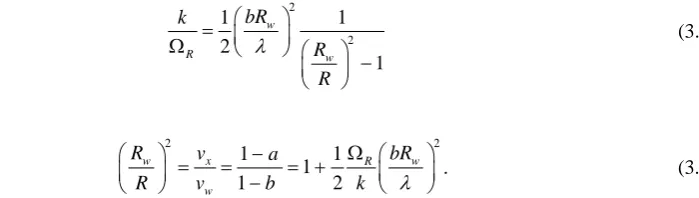
2, i.e., Equation (3.11) is not generally valid. Formula (3.34) was already derived by Wilson and Lissaman [62] for a propeller-type wind turbine; a similar formula was given by Glauert [10] for an engine-driven propeller. Obviously, Equation (3.34) can only be solved iteratively. Results of such a solution are shown inFigure 6. As illustrated, for tip speed ratios in the range of 0< <λ 0.25, the axial interference factor, a, becomes negative. These results have to be discarded because they disagree with observa-tions. For tip speed ratios λ≥2, the condition b=2a, derived in the matter of the axial momentum theory, is nearly fulfilled [10] [62]. From Equation (3.34) we can infer that the condition b=2a is exactly fulfilled if λ becomes infinite.In accord with Equation (2.54), the torque, dQ, experienced by this annular stream tube element between r and r+dr reads
2
(
)
dQ=ρ ωvx r dA=2πρv∞ 1−a kr rd , (3.36) where the area of the stream tube element is dA=2π dr r, and k is given by Equation (3.26). Since the power caused by the rotor is the product of the angular velocity and this annulus torque, i.e., dP= ΩRdQ, the integra-tion over the total blade span provides
(
)
2π 1 R
P= ρv∞ −a Ω kR . (3.37) Replacing ΩRk with the aid of Equation (3.33) yields
3 2
(
)
22 1
1 2
b a
P R v
b a
π ρ ∞ − =
− . (3.38) Thus, in contrast to the axial momentum theory, the wind power efficiency is given by [60] [62]
(
)
2 2 3 2 1 1 π 2 P b a P C b aR ρv∞
−
= =
Figure 6. Effect of the tip speed ratio λ, defined by Equation (3.35), on the induced velocities for flow with an irrotational
wake. The diagram on the right side is based onFigure 3.3 of Wilson and Lissaman [62]. Inserting b=2a into this formula provides Equation (3.22). This means that the power efficiency for the ir-rotational wake tends to that for the axial momentum theory (see Equation (3.22)) if the tip speed ratio exceeds
2
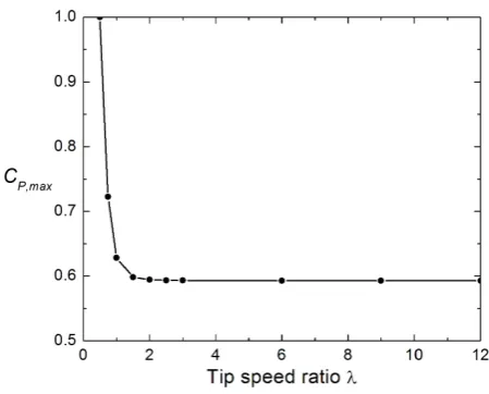
λ= [62] [65]. Since the ratio a b varies with λ (Figure 6), different tip speed ratios provide different curves for the power efficiency. The maximum power efficiency that is close to the Betz-Joukowsky limit of 0.593 occurs around b=2 3 if the tip speed ratio exceeds λ=2 (cf. Figure 7). Thus, for X =v w v∞ = −1 b we obtain X =1 3. This is the value for which the Betz-Joukowsky limit was determined (see Figure 5 and
Figure 7). Consequently, in case of an irrotational wake, the axial momentum theory provides reasonable results for tip speed ratios larger than λ=2.
Glauert [10] already argued:
The condition of constant circulation k along the blade, which has been the basis of the preceding calcula-tions, cannot be fully realized in practice since it implies that near the roots of the blades the angular velocity imparted to the air is greater than the angular velocity of the propeller itself. In any practical application of the analysis it is therefore necessary to assume that the effective part of the propeller blades commences at a radial distance not less than k ΩR at which ω is equal to ΩR.
It implies that, near the roots of the blades, the angular velocity imparted to the air is greater than the angular velocity of the propeller itself [6]. Wilson & Lissaman [62] and de Vries [40] shared Glauert’s viewpoint that the solution is unphysical as it results in infinite values of power and circulation when the tip-speed ratio tends to zero.
From Equations (3.30) and (3.33) we can derive
2
2
1 1
2
1
w
R w
bR k
R R
λ
=
Ω −
(3.40)
or
2 2
1 1
1
1 2
w x R w
w
R v a bR
R v b k λ
Ω −
= = = +
−
. (3.41)
The maximum values of the power efficiency for various tip speed ratios are also illustrated inFigure 8. This diagram shows that for λ<2 the maximum power efficiency notably exceeds the Betz-Joukowsky limit. However, these results must be assessed with care. For λ=0.5, for instance, we obtain CP,max =1 that occurs
at b=1. According to Figure 6, for b=1 the axial interference factor amounts to a=0. Consequently,
(
1)
x
![Figure 2. Turbulence intensity depending on wind speed at 90 m height for the period September 2003-August 2007 (taken from Türk and Emeis, [41])](https://thumb-us.123doks.com/thumbv2/123dok_us/8026458.767524/8.595.150.469.398.680/figure-turbulence-intensity-depending-height-period-september-august.webp)
![Figure 4. (a) Sketch of the stream-tube model; (b) Wind speed and pressure variations by approaching and leaving the rotor area (with respect to Betz [58])](https://thumb-us.123doks.com/thumbv2/123dok_us/8026458.767524/13.595.88.536.82.259/figure-sketch-stream-pressure-variations-approaching-leaving-respect.webp)
![Figure 5. The Betz-Joukowsky limit. The solid line represents Equation (3.17) and the dash-dotted lines characterize the maximum of the power efficiency (with respect to Betz [58])](https://thumb-us.123doks.com/thumbv2/123dok_us/8026458.767524/15.595.201.426.85.273/figure-joukowsky-represents-equation-characterize-maximum-efficiency-respect.webp)
![Figure 11. Sketch of the vortex system corresponding to lifting line theory of the ideal pro-peller of (a) Joukowsky and (b) Betz (from Okulov and Sørensen [12], but with respect to Sørensen [6])](https://thumb-us.123doks.com/thumbv2/123dok_us/8026458.767524/22.595.145.483.519.692/figure-sketch-corresponding-lifting-joukowsky-sorensen-respect-sorensen.webp)
![Figure 13N → ∞b [12]. Since neither the axial interference factor , where in both models tend towards the Betz-Joukowsky limit nor explicitly occurs in Equations (3.60) and (3.63), for various num-ber of blades depends on the tip-speed ratio number of](https://thumb-us.123doks.com/thumbv2/123dok_us/8026458.767524/24.595.139.485.453.677/figure-interference-joukowsky-explicitly-equations-various-depends-number.webp)
