Multicriteria Optimization of Cellular Networks

(1)

Multicriteria Optimization of Cellular Networks

Roman Statnikov1,2, Josef Matusov1, Kirill Pyankov3, Alexander Statnikov4

1_{Institute of Machines Science Named after A. A. Blagonravov of the Russian Academy of Sciences, Moscow, Russia} 2_{Department of Information Sciences, Naval Postgraduate School, Monterey, USA}

3_{Central Institute of Aviation Motors Named after P. I. Baranov, Moscow, Russia}

4_{Center for Health Informatics and Bioinformatics, New York University Medical Center, New York, USA}

Email: [email protected]

Received May 28, 2013; revised June 25, 2013; accepted July 9, 2013

Copyright © 2013 Roman Statnikov et al. This is an open access article distributed under the Creative Commons Attribution License, which permits unrestricted use, distribution, and reproduction in any medium, provided the original work is properly cited.

ABSTRACT

When designing modern cellular networks, it is challenging to account for many contradictory criteria and constantly changing external conditions of the networks (e.g., traffic). We need to solve multicriteria problems with high-dimensional vectors of parameters. A prerequisite to solution of these problems is correct determination of the feasible solution set, which is directly related to the statement of optimization problem. This is a major challenge in all multicriteria engineering optimization problems and represents significant difficulties for the expert. In this paper, we show how to define the feasible solution set for cellular network optimal design problems and thus answer the fundamental question of where to search for optimal solutions in such problems. We use the Parameter Space Investigation (PSI) method im- plemented in the Multicriteria Optimization and Vector Identification (MOVI) software system and apply it to a mathematical model of cellular network. In addition to developing methodology for stating and solving the problem of multicriteria optimization of cellular network, we have found that 1) defining the feasible solution set is directly related to the correct statement of the optimization problem, 2) once the feasible solution set has been determined, the criteria convolution can be applied to find the optimal solution in the feasible solution set, 3) it is possible to perform online tuning of the cellular network parameters.

Keywords: Feasible Solution Set; Pareto Optimal Solutions; Parameter Space Investigation (PSI) Method; Cellular Networks; Multicriteria Problems

1. Introduction

One of the distinguishing characteristics of cellular networks is difficulty of their design given a large number of contradictory criteria and constantly changing external conditions of the networks (e.g., traffic). In addition to multiple criteria, we deal with vectors of parameters of high dimensionality (hundreds to thousands). Optimal design of cellular networks is at the interface of design and management problems, and there have hardly been any attempts to construct a feasible solution set for problems of such type. The feasible solution set is essential because it contains a Pareto set of optimal solutions, none of which can be improved along all quality criteria simultaneously. In addition to the difficulties in determining the feasible solution set, choice of the best solution from a Pareto set is also non-trivial when this set contains a large number of solutions. In some cases, these difficulties can be mitigated by applying criteria convolution as described below. However, in order to

apply convolutions correctly, one has to define feasibility of obtained solution first, which makes a proper construction of the feasible solution set the key factor. In this work, we consider applying the Pareto Space Investiga- tion (PSI) method as an attempt to improve existing techniques of network design and management by con-structing and analyzing the feasible solution set. The goal of this paper is to show feasibility and capabilities of the PSI method for solving problems of optimal design of cellular networks.

Most existing works on cellular network optimization that deal with multi-criteria problems transform them into single-objective variant using some scalarization techniques [1,2], weighted sum being the most popular approach. Melachrinoudis and Rosyidi [3] use simulated annealing algorithm to optimize weighted sum of three criteria (call quality, demand coverage and total cost) by varying location, power and antenna height of base stations. Galota et al. [4] choose positions of base stations

(2)

supplied demand nodes, ongoing costs, and cost of in- tra-cell interference) subject to constraint on construction costs. Amaldi et al. [5] aim at maximizing total covered

traffic and minimizing total installation costs by forming weighted sum of these criteria; two-stage Tabu Search algorithm is used starting from solution provided by randomized greedy procedure. Hurley [6] proposes framework based on Simulated Annealing for optimization of objective function that is sum of five criteria (coverage, site cost, traffic, interference, and handover). Gerdenitsch [7] uses sum of number of served users, coverage, and soft handover as objective function for the problem of tuning transmit power and antenna downtilt using Genetic Algorithm. Zhu and Buot [8] propose heu- ristic algorithm for online network optimization based on estimating linear model between KPIs (key performance indicators) and parameters (expressed in form on sensi- tivity matrix) from a-priori simulation results and KPI measurements. Weighted sum of five KPIs is used as optimization process performance index. The approach allows specifying KPI targets.

In few works ε-constraint technique is utilized: one of criteria is selected to be optimized, and others are con- verted into constraints [1,2]. One of network optimization problems studied by Siomina [9] is example of such approach: total network load (total pilot power) is minimized subject to coverage constraint. Other approaches not based on some form of scalarization (weighted sum or ε-constraint) are much less common. Jedidi et al. [10]

argue that it makes sense to consider cells overlap and cells geometry as criteria for real-life network optimization. They aim at finding the whole Pareto front of this bi-criteria problem using a version of Multiobjective Evolutionary Algorithm. It is well known that such algorithms are quite effective for two or three criteria problems, as higher number of criteria their applicability is an open question [11]. To the best of our knowledge, most commercial cellular network planning and optimization tools are also based on some form of scalarization such as weighted sum [12,13].

2. Problem Formulation

In this paper, we are concerned with multicriteria optimization problems arising during planning and operation of cellular mobile network. Mobile network provides service in area divided into cells, each served by trans- ceiver of base station that has several tunable parameters affecting network performance like transmit power, antenna orientation, associated radio frequency, parameters of radio resource management algorithms, etc. Typically these parameters are configured by experts (possibly with the help of network planning and optimization tools) during network planning stage and kept fixed for a long period of time. Cellular network demand and environ-

ment are ever changing during day, and such fixed configuration (usually targeted at peak network load-busy hour) can become not well suited for current network conditions. It is also possible to change some of cellular network parameters online trying to adapt to changing conditions. Thus network optimization can be performed in offline (with full set of parameters available for configuration and lots of time for decision making) or online (with restricted set of parameters available and limited time for decision making) mode. We propose using of the Parameter Space Investigation method in both of the network optimization modes.

Reference signal transmit power and antenna electrical downtilt are one of the most important parameters that have great impact on different network KPIs such as capacity and coverage. Moreover, these two parameters can be changed remotely and automatically as opposed to manual and costly reconfiguration of some other important parameters (such as antenna azimuth or mechanical downtilt). This is the motivation for using the above two parameters for our study.

Whole network area is divided into pixels using some grid (typical size is 50 m  50 m), each pixel is characterized by receive power level from each cell in network and mean number of users in it. The former aggregates into signal propagation maps (one for each cell), and the latter into traffic map (traffic maps can be differentiated by type of service). Reference signal received power is reference signal transmit power times channel gain between cell and pixel, influenced by antenna downtilt of this cell. Increasing transmit powers of all cells and pointing antennas up (corresponds to small downtilt values), we increase coverage in network (received power in each pixel becomes high enough to connect to the cell with strongest signal) but at the same time we increase interference between cells, which effectively leads to network capacity degradation. Trade-off between these objectives is not obvious, and needs to be carefully studied. It is hard to say beforehand what KPI values are achievable [12-15].

2.1. System Model

Let us denote by c = 1, …, С the set of cells serving

planning area represented by a grid of pixels. Signal propagation (averaged in time and frequency) from each cell c to each pixel m is characterized by power gain gmcAmc, composed of isotropic gain gmc and antenna gain Amc. Antenna gain Amc depends on electrical downtilt tc of

antenna associated with cell c and direction (given by

azimuth mc and elevation mc angles) between this an-

tenna and pixel m: Amc G Hc c



tc,mc

 

V tc c,mc



,

where Gc is cell’s c antenna maximum gain, Hc

 

 ,

(3)

vertical cell c antenna patterns [14].

Reference Signal Received Power (RSRP) Rmc from

cell c in pixel m is calculated as

mc c mc mc

R P g A ,

where Pc is reference signal transmit power of cell c.

Each pixel m is associated with cell c with largest re-

ceived power Rmc among all other cells, for such pixel–

cell pair m, c we set association indicator amc equal to 1.

Signals from all other cells interfere with useful signal from serving cell. One of the most important link quality indicators is Reference Signal Signal-to- Interference and Noise Ratio (RSSINR) given by

2 \{ } mc mc md d c R R   _  



_ ,

where _2_{is noise power.}

Each cell has frequency resources (resource blocks in LTE) that it allocates between served users. We use definition of cell load as long-term average percentage of utilized frequency resources [16]. Cell load depends on amount of traffic requested by served users and their link capacities. We characterize long-term average requested traffic in pixel m using Tm—average number of users in

this pixel requesting some service, and D—bitrate demand

of this service. Load of cell c required to serve its users is

estimated as





2 log 1 mc m c m c m a T D W  c   



,

where Wc is bandwidth of frequency resources available

in cell c. Here we used Shannon formula for link capaci-

ties.

2.2. Performance Criteria

Call Drop and/or Block Rate (CDBR) performance criterion CDBR is determined by cell loads and number of

served users as





1 CDBR

max 0,1 1/ c m

c m mc c m a a      



 

c .

Percentage of RSRP and RSSINR covered area criteria

RSRP-covA and RSSINR-covA are defined as



0



2 RSRP-covA , mc mc c m mc c m

a h R R

a

   

 

and



0



3 RSSINR-covA , mc mc c m mc c m a h a      

 

,

where 0 and

R 0 are RSRP and RSSINR thresholds

and

 

0

0 1

,

0 otherwise

x x h x x   

 . In a similar way per-

centage of RSRP and RSSINR covered traffic criteria criteria RSRP-covT and RSSINR-covT are defined as



0



4 RSRP-covT

mc mc c m

c m

a T h

  mc,

mc mc

R R

a T

 

 

and



0



5 RSSINR-covT

mc c m

c m

a T_m _mc,

mc m

h

a T

 

   

 

. Mean SINR

(Signal to Interference and Noise Ratio) [dB] KPI is de-fined as

 

6 M-SINR 10

10

log

mc m mc

c m m m a T T     

 



.

Mean required cell load criterion is

7 M-load

c c

C

   



 . Aggregated criterion is weighted

sum of the above seven criteria _aggr 7 . Usually

1

i i i  





cellular network operator has well-defined targets that should be achieved for RSRP-covA, RSRP-covT, and CDBR criteria, and additionally we would like to maxi- mize/minimize the following criteria shown in Table 1.

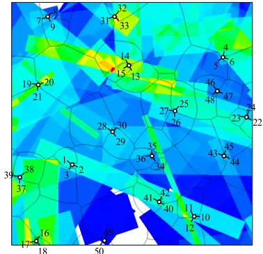
In our examples, we consider network consisting of 50 cells with 100 variables. Variables are transmit power pc

and electrical downtilt tc, c = 1, ..., 50. The considered

network with traffic map is shown in Figure 1. In the

1 2 3

4 5 6

7 8 9 10 11 12 13 14 15 16 17 18 19 20 21 22 23 24 25 26 27 28 29 30 31 32 33 34 35 36 37 38 39 40 41 42

[image:3.595.327.516.443.625.2]

43 44 45 46 47 48 49 50

(4)

[image:4.595.55.547.101.239.2]

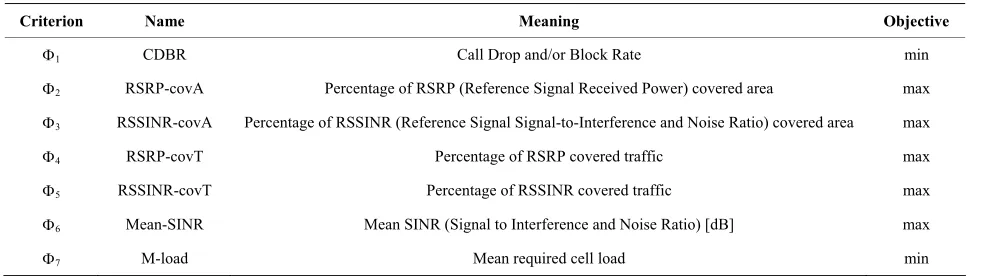
Table 1. Criteria names, meaning and objective.

Criterion Name Meaning Objective

1 CDBR Call Drop and/or Block Rate min

2 RSRP-covA Percentage of RSRP (Reference Signal Received Power) covered area max

3 RSSINR-covA Percentage of RSSINR (Reference Signal Signal-to-Interference and Noise Ratio) covered area max

4 RSRP-covT Percentage of RSRP covered traffic max

5 RSSINR-covT Percentage of RSSINR covered traffic max

6 Mean-SINR Mean SINR (Signal to Interference and Noise Ratio) [dB] max

7 M-load Mean required cell load min

There also exist particular performance criteria. It is

desired, all other things being equal, these criteria, denoted by Φ_

 

 , 1,.., ,k take the extreme values. For simplicity, we assume that 

 

 are to be mini-

mized. first problem (Task 1), 0  pc  40 W, 0˚  tc  10˚ of

each cell, c = 1, ..., 50. In the second problem (Task2),

0  pc  50 W. The ranges of change for the electrical

downtilt are kept unchanged by 0˚tc 10˚ of each cell, c = 1, ..., 50. Electrical downtilt constraints are

deter-mined by capabilities of antennas serving each cell. Transmit power constraints are also due to hardware limitations (power amplifier) and electromagnetic radia-tion regularadia-tions.

The constraints (1) single out a parallelepiped  in the

r-dimensional design variable space (space of design

variables).

In order to avoid situations, in which the expert re- gards the values of some criteria as unacceptable, we introduce the criteria constraints

In what follows we will show how to construct the feasible solution set for the above set of performance

criteria.

_{ }

_, _1,..,_k

   

    , (3)

3. Construction of the Feasible and Pareto

Optimal Solution Sets

where

**

 is the worst value of the criterion 

 



to which the expert may agree. The choice of 

 

 is

discussed in what follows.

3.1. Generalized Formulation of Multicriteria

Optimization Problems The criteria constraints differ from the functional con-

straints in that the former are determined when solving a problem and, as a rule, are repeatedly revised. Hence, unlike Cl

_and

l

C, reasonable values of  cannot

be chosen before solving the problem. We discuss here a mathematical formulation that can be

applied to the majority of engineering optimization problems [17-23]. In the general case, when designing a system, one has to take into account the design variable constraints, the functional constraints, and the criteria constraints.

Constraints (1)-(3) define the feasible solution set D. If the functions fl() and 

 

 are continuous in ,

then the sets G and D are closed.

Now let us formulate one of the basic problems of multicriteria optimization. It is necessary to find such a set PD for which

The design variable constraints (constraints on the

de-sign variables) have the form:

(1) , 1, ,

j j j j r

_ _ _ _ _.

,



 

min



D

P

 



   (4)

The functional constraints on functional dependences fl() may be written as follows:

(2)

 

, 1, ,

l l l

C f  C l  t

where 

 

  



₁

 

 ,₂

 

 , ...,_k

 





is the criterion vector and P is the Pareto optimal set.

In other words, a point , is called a Pareto optimal point if there exists no point

0

D

 

D

 such that

 

0

   

   for all  = 1, …, k and

 

0

0 0

   

   for at least one  {1, …, k}. A set P D is called the Pareto optimal set iff it consists of

Pareto optimal points. where l and l are, respectively, the lower and the

upper admissible values of the quantity fl(). Conditions

(2) often represent compliance with standard regulatory requirements to the system. As a rule, vectors of design variables

r

C C

,



1 2,...,

     are calculated using uni- formly distributed sequences. In the present case, a ran- dom number generator was applied because of high dimensionality of the design variable space.

(5)

cause, by definition, the optimal vector always belongs to the Pareto optimal set, irrespective of the system of pref- erences used by the expert for comparing vectors be- longing to the feasible solution set.

Very often, the experts do not encounter serious difficulties in analyzing the feasible solution set and the optimal set and in choosing the most preferred solution. They have a sufficiently well-defined system of prefer- ences. Moreover, the aforementioned sets usually contain a small number of elements [17,23].

3.2. The PSI Method

To formulate and solve engineering optimization problems, the Parameter Space Investigation (PSI) method has been developed. According to this method, in the process of dialogues with a computer, the expert deter- mines the criteria constraints and performs multicriteria analysis. The PSI method gives the expert valuable information on the advisability of revising various criteria, functional, and design variable constraints with the aim of improving the basic criteria. The expert sees what price one pays for making concessions in various criteria,

i.e., what one loses and what one gains. In other words,

the expert corrects initial problem statement while solving it, analyses the feasible solution set, and then makes a decision. A systematic and comprehensive description of the method can be found in [17,21,23].

After analyzing P (Pareto optimal set), the expert finds

the most preferred solution _₍_0₎_{. Typically, for the}

problems under consideration, experts do not have serious difficulties in analyzing the Pareto optimal set and in

choosing the most preferred solution. Thus, the PSI method has proved to be a very convenient and effective tool for the expert, primarily because this method can be directly used for the statement and solution of the problem in an interactive mode. The PSI method is imple-

mented in the Multicriteria Optimization and Vector Identification (MOVI) software system [17].

It is also worth mentioning that while there are many optimization methods, the PSI method more fully ad- dresses characteristics of real-world engineering optimization problems (e.g., multiple criteria, difficulties in determining constraints on design variables, functional dependences and criteria) and allows the expert to simultaneously formulate and solve them in an interactive mode.

4. Application of the PSI Method to

Improving the Network

The PSI method has been applied to the mathematical model of the network described above. Recall that in the above two examples, we have 50 cells with 100 variables and the number of criteria is seven. As test examples, we solve Task 1 and Task 2, that differ in maximum allowed transmit power—40 W and 50 W, respectively.

4.1. Test Tables for Task 1 (40 W)

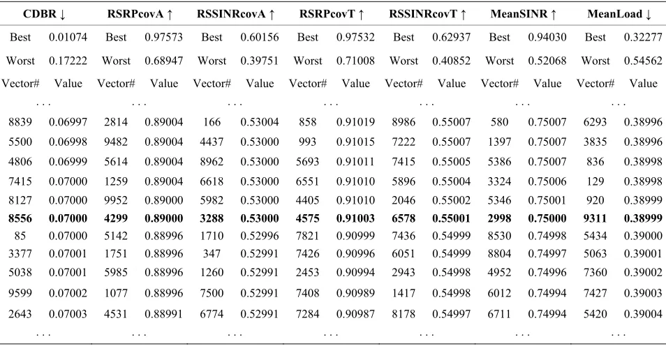
[image:5.595.60.537.489.737.2]

As follows from the PSI method, the criteria constraints should be determined first. We have constructed the test table after 10,000 tests, see Table 2. The list of criteria, the best and worst values of criteria are shown in the

Table 2. Fragment of the tеst tables (Criteria that maximized and minimized are denoted with  and , respectively). CDBR ↓ RSRPcovA ↑ RSSINRcovA ↑ RSRPcovT ↑ RSSINRcovT ↑ MeanSINR ↑ MeanLoad ↓

Best 0.01074 Best 0.97573 Best 0.60156 Best 0.97532 Best 0.62937 Best 0.94030 Best 0.32277

Worst 0.17222 Worst 0.68947 Worst 0.39751 Worst 0.71008 Worst 0.40852 Worst 0.52068 Worst 0.54562

Vector# Value Vector# Value Vector# Value Vector# Value Vector# Value Vector# Value Vector# Value

      

8839 0.06997 2814 0.89004 166 0.53004 858 0.91019 8986 0.55007 580 0.75007 6293 0.38996 5500 0.06998 9482 0.89004 4437 0.53000 993 0.91015 7222 0.55007 1397 0.75007 3835 0.38996 4806 0.06999 5614 0.89004 8962 0.53000 5693 0.91011 7415 0.55005 5386 0.75007 836 0.38998 7415 0.07000 1259 0.89004 6618 0.53000 6551 0.91010 5896 0.55004 3324 0.75006 129 0.38998 8127 0.07000 9952 0.89000 5982 0.53000 4405 0.91010 2046 0.55002 5346 0.75001 920 0.38999 8556 0.07000 4299 0.89000 3288 0.53000 4575 0.91003 6578 0.55001 2998 0.75000 9311 0.38999 85 0.07000 5142 0.88996 1710 0.52996 7821 0.90999 7436 0.54999 8530 0.74998 5434 0.39000 3377 0.07001 1751 0.88996 347 0.52991 7426 0.90996 6051 0.54999 8804 0.74997 5063 0.39001 5038 0.07001 5985 0.88996 1260 0.52991 2453 0.90994 2943 0.54998 4952 0.74996 7360 0.39002 9599 0.07002 1077 0.88996 7500 0.52991 7408 0.90989 1417 0.54998 6012 0.74994 7427 0.39003 2643 0.07003 4531 0.88991 6774 0.52991 7284 0.90987 8178 0.54997 6711 0.74994 5420 0.39004

(6)

first, second and third rows, respectively. As a result of the dialogues of computer with the expert, the criteria constraints (0.07000; 0.89000; 0.53000; 0.91003; 0.55001; 0.75000; 0.38999) have been determined, see Table 2. We have obtained 256 feasible solutions, including 50 Pareto optimal solutions. Since these constraints met the expert’s requirements, they have been accounted for in all further studies. These constraints were identical in Task 2 (50 W), where we have conducted 10,000 tests and obtained 2867 feasible solutions, including 95 Pareto optimal solutions.

4.2. Criteria Histograms for Task 1

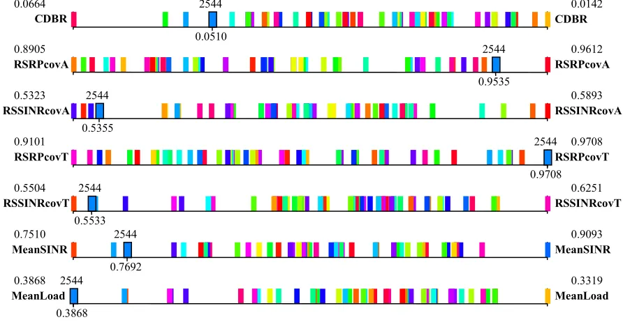
[image:6.595.74.520.490.721.2]

Criteria histograms are constructed on the basis of test tables and allow us to make a decision based on the obtained values of the criteria vectors and their significance [17,23]. In particular, the histograms allow us to correct the initial problem statement and reveal criteria relations. Histograms show Pareto optimal vectors for all criteria (e.g., see Figure 2). For each criterion, a horizontal line is assigned, along which vertical bars are plotted. Each bar corresponds to a vector from the Pareto optimal set. The location of each bar is defined by a corresponding criterion value for this vector. Criterion name as well as the worst and best criterion values are displayed to the left and to the right of the corresponding horizontal band, respectively.

Figure 2 shows locations of all 50 Pareto optimal vectors within obtained constraints on their values. Each of 50 solutions is uniquely colored. As can be seen, improving some criteria leads to deterioration of the others. For example, Pareto optimal solution #2544 is the

best according to the fourth criterion (RSRP- ,

2544 4

Φ = 0.9708) and one of the best according to the second criterion (RSRP A, 2544

2

Φ = 0.9535) however it is the worst according to the seventh criterion (M-

2544 7

Φ = 0.3868) and one of the worst according to the third (RSSINR-covA 4

3 = 0.5355), fifth

(RSSINR-covT, = 0.5533), and sixth (Mean- SINR, = 0.7692) criteria, (see Figure 2). These histograms demonstrate complex relationships that exist between the criteria.

covT

-cov

, load,

254

Φ

2544 5

Φ

2544 6 

4.3. Search for Optimal Solutions by

Optimization of the Criteria Aggregate

In our case, the biggest challenges for an expert included the choice of a preferred solution from the Pareto optimal set: there were 50 and 95 Pareto optimal solutions in Task 1 and Task 2, respectively. As mentioned above, an expert defined an objective function as an aggregate of criteria

7

aggr 1

, i i i

 

 





where 1 = 0.2, 2 = –0.2, 3 = –0.1, 4 = –0.2, 5 = –0.1,

6 = –0.1, and 7 = 0.1. The search for optimal solution

was performed on the feasible set which is defined by constraints on parameters and criteria. For Task 1, the minimal value of the criteria aggregate (see [24]) was –0.6226, with the vector of criteria (0.0072; 0.9804; 0.6803; 0.9827; 0.7207; 1.1813; 0.2676). For Task 2, the minimal value of the criteria aggregate was –0.6262 with the vector of criteria (0.0108; 0.9748; 0.6825; 0.9819; 0.7275; 1.2209; 0.2612).

2544

0.0510

CDBR CDBR

0.0664 0.0142

2544

0.9535

RSRPcovA RSRPcovA

0.8905 0.9612

2544

0.5355

RSSINRcovA RSSINRcovA

0.5323 0.5893

2544

0.9708

RSRPcovT RSRPcovT

0.9101 0.9708

2544

0.5533

RSSINRcovT RSSINRcovT

0.5504 0.6251

2544

0.7692

MeanSINR MeanSINR

0.7510 0.9093

2544

0.3868

MeanLoad MeanLoad

0.3868 0.3319

(7)

5. Conclusions

this work are three-fold. First,

defin-(National Re-

REFERENCES

[1] K. Miettinen, imization,”

iettinen and R. Slowinski,

“Mul-The conclusions of

ing the feasible solution set is directly related to the correct statement of the optimization problem for the cellular network. We developed methodology for stating and solving the problems of multicriteria optimization for cellular network and showed how to state and solve the multicriteria problem of construction of the feasible and Pareto optimal solution sets.

Second, as it is known, the most preferable solution is determined on the Pareto set. In order to find it, one has to determine feasible solution set. Determination of the latter, correct definition of criteria constraints, turned out to be a difficult problem. These constraints were determined as a result of dialogues between an expert and compute while analyzing the test tables. Analysis of the Pareto optimal set is also challenging for the expert because of a large number of Pareto solutions. To overcome this, we have used a convolution of criteria. It is worth- while to note that only after the feasible solution set has been determined, the criteria convolution can be suc- cessfully applied to find the optimal solution.

Third, to tune the network parameters online, i.e. to

account for real distribution of the traffic, the operator may reduce the time required for the analysis. This process can be automated.

6. Acknowledgements

The authors are grateful to M. Pikhletsky

search University “Moscow Power Engineering Institute”) for participation in the problem formulation. The authors would like to thank A. Isyanov (Central Institute of Avi- ation Motors) for his contribution to computational ex- periments.

“Nonlinear Multiobjective Opt Kluwer, Boston, 1999.

[2] J. Branke, K. Deb, K. M

tiobjective Optimization: Interactive and Evolutionary Approaches,” Springer-Verlag, Berlin, 2008.

doi:10.1007/978-3-540-88908-3

[3] E. Melachrinoudis and B. Rosyidi, “Optimizing the De- sign of a CDMA Cellular System Configuration with Multiple Criteria,” Annals of Operations Research, Vol. 106, No. 1-4, 2001, pp. 307-329.

doi:10.1023/A:1014574028174

[4] M. Galota, C. Glaßer, S. Reith and H. Vollmer, “A

Poly-[5] E. Amaldi, P. Belotti, A. Capone and F. Malucelli, “Op- tion and Configuration in UMTS erations Research

nomial-Time Approximation Scheme for Base Station Positioning in UMTS Networks,” Proceedings of the 5th International Workshop on Discrete Algorithms and Me- thods for Mobile Computing and Communications, Rome, 21 July 2001, pp. 52-59.

timizing Base Station Loca

Networks,” Annals of Op , Vol. 146, No. 1, 2006, pp. 135-151. doi:10.1007/s10479-006-0046-3 [6] S. Hurley, “Planning Effective Cellular Mobile Radio

Networks,” IEEE Transactions on Vehicular Technology, Vol. 51, No. 2, 2002, pp. 243-253.

doi:10.1109/25.994802

[7] A. Gerdenitsch, “System Capacity Optimization of UMTS FDD Networks,” PhD Thesis, Te

Wien, Wien, 2004.

chnische Universitat

9 May 2004, pp. 2370-2374.

Methods for WCDMA Radio Net- issertation, erlag,

Wies-versitat Berlin, Berlin, 2008.

don, 2002. doi:10.1007/978-94-015-9968-9 [8] H. Zhu and T. Buot, “Multi-Parameter Optimization in

WCDMA Radio Networks,” Vehicular Technology Con- ference, Milan, 17-1

[9] I. Siomina, “Radio Network Planning and Resource Op- timization: Mathematical Models and Algorithms for UMTS, WLANs, and Ad Hoc Networks,” PhD Disserta-tion, Linkoping University, Linkoping, 2007.

[10] A. Jedidi, A. Caminada and G. Finke, “2-Objective Opti- mization of Cells Overlap and Geometry with Evolution- ary Algorithms,” Applications of Evolutionary Computing, Lecture Notes in Computer Science, Vol. 3005, 2004, pp 130-139.

[11] V. Khare, X. Yao and K. Deb, “Performance Scaling of Multi-Objective Evolutionary Algorithms,” Proceedings of the Second Evolutionary Multi-Criterion Optimization (EMO-03) Conference (LNCS 2632), Faro, 8-11 April 2003, pp. 376- 390.

[12] Symena Software and Consulting GmbH. “CAPESSO 14.3 User Manual,” 2011.

[13] Forsk SA, “Atoll 2.8.3-User Manual,” 2010. [14] U. Turke, “Efficient

work Planning and Optimization,” PhD D TeubnerVerlag and DeutscherUniversitats-V baden, 25 September 2007.

[15] H. F. Geerdes, “UMTS Radio Network Planning: Mas- tering Cell Coupling for Capacity Optimization,” PhD Dissertation, Technische Uni

[16] K. Majewski and M. Koonert, “Conservative Cell Load Approximation for Radio Networks with Shannon Chan- nels and Its Application to LTE Network Planning,” IEEE Sixth Advanced International Conference on Telecommu- nications, Barcelona, 9-15 May 2010.

[17] R. Statnikov and A. Statnikov, “The Parameter Space In- vestigation Method Toolkit,” Artech House, Boston/Lon- don, 2011.

[18] R. Statnikov and J. Matusov, “Multicriteria Analysis in Engineering,” Kluwer Academic Publishers, Dordrecht/ Boston/Lon

[19] R. Statnikov and J. Matusov, “Multicriteria Optimization and Engineering,” Chapman & Hall, New York, 1995. doi:10.1007/978-1-4615-2089-4

(8)

rameters in Multicriteria Problems,” 2nd Edition, Drofa, Moscow, 2006 (in Russian).

[22] R. B. Statnikov and J. B. Matusov, “Use of Nets for the Approximation of the Edgeworth-Pareto Set in Multicri-teria Optimization,” Journal of Optimization Theory and Application, Vol. 91, No. 3, 1996, pp. 543-560.

doi:10.1007/BF02190121

[23] R. Statnikov, J. Matusov and A. Statnikov, “Mu Engineering Optimization Probl

and Applications,” Journal of Optimization Theory and Applications, Vol. 155, No. 2, 2012, pp. 355-375. doi:10.1007/s10957-012-0083-9

[24] B. Suman and P. Kumar, “A Survey of Simulate nealing as a Tool for Single and Multiobjective Optimiza- d An- tion,” Journal of the Operational Research Society, Vol. 57, 2006, pp. 1143-1160.

doi:10.1057/palgrave.jors.2602068 lticriteria