Magnitude and variability of land evaporation and its components at the global scale

www.hydrol-earth-syst-sci.net/15/967/2011/ doi:10.5194/hess-15-967-2011

© Author(s) 2011. CC Attribution 3.0 License.

Earth System

Sciences

Magnitude and variability of land evaporation and its components

at the global scale

D. G. Miralles1, R. A. M. De Jeu1, J. H. Gash1, T. R. H. Holmes1,2, and A. J. Dolman1 1_{Department of Hydrology, VU University, Amsterdam, The Netherlands}

2_{Hydrology and Remote Sensing Lab, USDA-ARS, Beltsville, MD, USA}

Received: 10 December 2010 – Published in Hydrol. Earth Syst. Sci. Discuss.: 3 January 2011 Revised: 11 March 2011 – Accepted: 14 March 2011 – Published: 17 March 2011

Abstract. A process-based methodology is applied to esti-mate land-surface evaporation from multi-satellite informa-tion. GLEAM (Global Land-surface Evaporation: the Am-sterdam Methodology) combines a wide range of remotely-sensed observations to derive daily actual evaporation and its different components. Soil water stress conditions are de-fined from a root-zone profile of soil moisture and used to estimate transpiration based on a Priestley and Taylor equa-tion. The methodology also derives evaporationfrom bare soil and snow sublimation. Tall vegetation rainfall intercep-tion is independently estimated by means of the Gash analyt-ical model. Here, GLEAM is applied daily, at global scale and a quarter degree resolution. Triple collocation is used to calculate the error structure of the evaporation estimates and test the relative merits of two different precipitation in-puts. The spatial distribution of evaporation – and its differ-ent compondiffer-ents – is analysed to understand the relative im-portance of each component over different ecosystems. An-nual land evaporation is estimated as 67.9×103km3, 80% corresponding to transpiration, 11% to interception loss, 7% to bare soil evaporation and 2% snow sublimation. Results show that rainfall interception plays an important role in the partition of precipitation into evaporation and water available for runoff at a continental scale. This study gives insights into the relative importance of precipitation and net radiation in driving evaporation, and how the seasonal influence of these controls varies over different regions. Precipitation is recog-nised as an important factor driving evaporation, not only in areas that have limited soil water availability, but also in ar-eas of high rainfall interception and low available energy.

Correspondence to: D. G. Miralles ([email protected])

1 Introduction

Despite the importance of latent heat flux as the link between water, carbon and energy cycles, land-surface evaporation re-mains one of the most uncertain terms in the world’s water balance (Dolman and de Jeu, 2010). Estimates of evapora-tion from land surface models and Global Circulaevapora-tion Mod-els (GCMs) differ greatly both in their global numbers (see Dirmeyer et al., 2006; Lim and Roderick, 2009) and their spatial distribution (Jim´enez et al., 2009). This creates the need for observation-based evaporation benchmark datasets to evaluate GCM performance (Blyth et al., 2009). Such datasets would help GCM developers to improve their evap-oration schemes and consequently their model predictions of future climate.

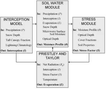
Fig. 1. Schematic overview of GLEAM (adapted from Miralles et al., 2011).

of forest rainfall interception (Gash, 1979; Valente et al., 1997).

GLEAM uses a broad range of independent remotely-sensed observations as a basis for estimating daily actual evaporation (and its different components) at a quarter-degree spatial resolution. The approach is based on the pa-rameterization of physical processes and although it contains some empirical parameters these have been derived from the results of separate field studies. The evaporation product has been successfully validated at site level over different vege-tation and climate conditions using in situ observations from 43 stations of the FLUXNET global network of micrometeo-rological flux measurements (see Miralles et al., 2011). The extensive use of observational data, the coupling between evaporation and soil moisture conditions and the separate estimation of rainfall interception allow application of the methodology in land-atmosphere feedback studies and tests of GCM performance.

Here, triple collocation (TC) is used to map the error of the evaporation estimates following the methodology in Miralles et al. (2010a). GLEAM is then applied at a watershed scale to validate the estimated long-term partitioning of incoming precipitation (P) into evaporation (E) and water available for runoff (P−E) using observations of river discharge from the Global Runoff Data Centre (GRDC). The methodology is fi-nally applied at a global scale to study the global distribution of land evaporation and its different components. The role of

rainfall interception and soil moisture on both the long-term partitioning of precipitation, and the seasonal distribution of the main drivers of evaporation (i.e. net radiation and precip-itation), are analysed in detailed.

2 Methodology 2.1 GLEAM

The model is driven by a large set of remote sensing obser-vations from different satellites (see Miralles et al., 2011, for a detailed description of the different input datasets and full details of the methodology). GLEAM produces daily esti-mates of land evaporation at a 0.25◦_{spatial resolution. It is}

structured in four interconnected units (see Fig. 1): (a) the interception model, (b) the soil water module, (c) the stress module, and (d) the PT module. The scheme is indepen-dently formulated for three land surface types with specific physical characteristics: (a) land covered by tall canopies, (b) land covered by short vegetation, and (c) bare soil.

component of GLEAM is described in detail by Miralles et al. (2010b).

The soil water module consists of a multilayer bucket model driven byP and calculating soil moisture for differ-ent layers within the root-zone. Satellite-measured surface soil moisture is assimilated into the first layer of the profile by means of a Kalman filter. The Kalman filter is based on the uncertainty of soil moisture observations, which is cal-culated using satellite-derived vegetation optical depth (the higher the optical depth, the higher the uncertainty in sur-face soil moisture – see De Jeu et al., 2008). Optimised es-timates of soil moisture (θ) are subsequently translated into estimates of evaporative stress represented by a factor (S), ranging from 0 (maximum stress) to 1 (no stress). PT esti-mates of potential evaporation are multiplied bySto estimate plant transpiration (in vegetated cover) and bare soil evap-oration. The final estimate of actual evaporation for each pixel is the result of aggregating the fluxes from the three different land cover types (tall canopy interception loss, tall canopy transpiration, short vegetation transpiration, bare soil evaporation) weighted by the percentage of each cover type within the pixel. In pixels covered by ice and snow,Eis inde-pendently calculated by adapting the PT equation to estimate sublimation as described by Murphy and Koop (2005). 2.2 Error analysis

A traditional way to estimate the uncertainty of model out-puts is through error propagation studies. These studies ac-count for the sensitivity of the output to uncertainties in the input data but do not give information on the quality of the model itself. Triple collocation (TC – Stoffelen, 1998; Sci-pal et al., 2008), however, allows the estimation of the en-tire error structure of the estimates of a model. This is done by simultaneously inter-comparing the product to two other datasets that observe the same physical phenomenon and present uncorrelated errors. Here, we are not only interested in the sensitivity of GLEAM estimates to errors in the set of inputs, but also in the uncertainties introduced by the param-eterization of the physical processes within the methodology. Consequently, an error analyses based on TC has been under-taken to evaluate the evaporation product.

Requirements for the application of TC are: (a) the three datasets must refer to the same physical phenomenon, (b) the number of triplets has to be large (i.e. sufficient time steps in which the three datasets report an estimate), and (c) errors of the different datasets must be uncorrelated. If these three requisites are fulfilled the estimated errors of a single product are not sensitive to the choice of the two other datasets (see Dorigo et al., 2010).

In order to meet the requirement of uncorrelated errors the products need to be mutually independent. To perform the TC-based evaluation of GLEAM, two (a priori) indepen-dent global daily evaporation datasets were selected: (a) the Princeton University product (Sheffield et al., 2010), and

(b) the Modern Era Retrospective-analysis for Research and Applications (MERRA) product. The Princeton University product is based on the application of a modified Penman-Monteith equation driven by a collection of satellite data. MERRA evaporation is a reanalysis product from NASA that uses the Goddard Earth Observing System Data Assimilation System (GEOS-5 DAS – Bosilovich, 2008).

The TC analysis presented here is limited to the spatial domain and the period (2003–2006) in which the three se-lected products overlap. Ideally, an infinite number of com-mon observations is required in the application of TC to ob-tain unbiased results. However, statistical tests revealed that a minimum number of 100 triplets is sufficient to allow the application of the method (Scipal et al., 2008).

A disadvantage of TC is that it does not retrieve any infor-mation about biases. Consequently – and in order to ease the interpretation of the results – the analyses presented here are based on characterising the error of the anomalies of evap-oration as calculated relative to a seasonally-varying clima-tology. Therefore the feature of GLEAM that is evaluated in this study is its skill in representing short-term changes in evaporation (e.g. after rainfall events), and how that skill changes from region to region. This error analysis follows closely the methodology presented in Miralles et al. (2010a) and Dorigo et al. (2010).

For each pixel, the three datasets are decomposed into cli-matology mean and anomaly components:

Ei = Ei0 + hEiND(i), (1)

where hEiN

D(i) is the climatological expectation for

land-surface evaporation at the day-of-year (D) associated with time stepi, andE_i0is the actual anomaly relative to this ex-pectation. Values ofhEiN

D(i) are calculated using a moving

window averaging of multi-year data with a window size of 31 days centered onD.

Subsequently, the time series of anomalies of the three products need to be scaled to the same dynamic range. This scaling is done by first selecting one of the datasets as the reference. Then the time series of the other two are nor-malised at every pixel to match the standard deviation of the time series of the reference one. To retrieve the errors within the dynamic range of GLEAM the dataset selected as refer-ence must be GLEAM. Note that the choice of the referrefer-ence dataset does not influence the relative magnitude of the errors of the three products at a given pixel.

TC assumes a linear relation between the three indepen-dent estimates of a physical variable and the hypothetical true value (Stoffelen, 1998). In our case the time series of anoma-lies of the three evaporation products (E_G0 for GLEAM,E_PU0 for the Princeton University product andE0_M for MERRA) can be expressed as a function of the hypothetical true evap-oration anomalies (E_TRUE0 ):

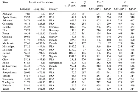
Table 1. GRDC stations used in the comparison ofP−Eand observed annual river runoff (Q). Results correspond to the period 2003–2006.

River Location of the station Area Q P−E E

(103km2) (mm) (mm) (mm) Lat (deg) Long (deg) Country CMORPH GPCP CMORPH GPCP

Alabama 7.80 6.77 USA 55.6 581 661 654 884 892

Apalachicola 29.95 −85.02 USA 49.7 443 515 596 895 910 Arkansas 34.79 −92.36 USA 409.3 83 405 115 735 647 Columbia 46.18 −123.18 USA 665.4 284 104 209 467 463 Danube 45.22 28.72 Romania 807.0 296 286 455 438 457 Elbe 53.23 10.89 Germany 132.0 151 216 450 321 347 Fraser 49.38 −121.45 Canada 217.0 361 194 369 468 514 Glomma 59.61 11.12 Norway 40.5 501 646 646 296 295 Liard 61.75 −121.22 Canada 275.0 284 136 160 380 390 Mackenzie 67.46 −133.74 Canada 1660.0 177 83 97 329 344 Mississippi 37.22 −89.46 USA 1847.2 81 369 199 523 487 Missouri 38.71 −91.44 USA 1357.7 37 322 120 521 468 Nelson 56.40 −94.37 Canada 1060.0 105 136 156 386 414 Niger 7.80 6.77 Nigeria 1331.6 125 381 156 368 327

Ohio 38.28 −85.80 USA 236.1 570 486 622 634 649

Rhine 51.84 6.11 Netherlands 160.8 378 253 520 408 440 St. Lawrence 45.42 −73.62 Canada 959.1 265 212 478 492 546

Snake 46.10 −116.98 USA 240.8 107 90 70 454 377

Susquehanna 39.66 −76.18 USA 70.2 697 421 761 579 630 Tanana 64.57 −149.09 USA 66.3 346 251 251 314 314 Tennessee 35.23 −88.26 USA 85.8 822 820 670 793 791 Tombigbee 31.76 −88.13 USA 47.7 641 712 566 929 932

Wabash 38.40 −87.75 USA 74.2 424 628 691 555 559

Yukon 61.93 −162.88 USA 831.4 254 178 179 314 314

E_PU0 = E0_TRUE +PU, (3)

E_M0 =E_TRUE0 +M, (4)

where G, PU and M are the residual errors relative to E_TRUE0 . Subtracting Eqs. (3) and (4) from Eq. (2) leads to

E_G0 −E0_PU = G −PU, (5)

E_G0 −E0_M = G − M. (6)

Multiplying Eqs. (5) and (6) and taking the average in time (indicated by ”h−i”) leads to

h(E0_G −E0_PU) (E0_G −E_M0 )i (7)

= h2_Gi − hGPUi − hGMi + hPUMi.

If the errors of the three datasets are uncorrelated the residual covariances can be assumed to be zero. Therefore Eq. (7) can be expressed as

h(E0_G −E0_PU) (E0_G −E_M0 )i = h_G2i. (8) The root mean square error (RMSE) of the GLEAM-estimated evaporation anomalies will therefore be

RMSE(E_G0, E0_TRUE)= q

h(E0_G −E0_PU) (E0_G −E_M0 )i. (9) The results of this TC error analysis are presented in Sect. 4.1.

3 Validation using river discharge

This validation at basin-scale of GLEAM evaporation esti-mates uses river discharge measurements from the Global Runoff Data Centre (GRDC) in Koblenz, Germany. It is complementary to the validations of the independent mod-ules described by Miralles et al. 2010b, 2011).

The study covers a period of 4 years (2003–2006). Cu-mulative GLEAM estimates ofP−E at 24 catchments are compared to observations of river runoff; the description of the river basins is presented in Table 1. Catchments were se-lected according to the availability of GRDC data during the complete study period and only rivers with an average annual discharge larger than 20 km3were considered for the study.

spatial domain (60◦_N–60◦_{S) does not cover the entire globe,}

and (b) precipitation is severely underestimated at higher lat-itudes during winter time (see Zeweldi and Gebremichael, 2009). Consequently, the 1◦resolution Global Precipitation Climatology Project (GPCP-1DD) product (Huffman et al., 2001) is used in GLEAM outside the CMORPH domain and when the temperature drops below 0◦C.

Due to the obvious sensitivity of theP−E estimates to uncertainties in P, this validation study is repeated using exclusively GPCP-1DD asP. Note that the choice of pre-cipitation product implicitly affects the calculation ofE in GLEAM. However, the sensitivity ofP−Eestimates toP will be higher than the sensitivity ofE estimates toP (this can also be noted in Table 1).

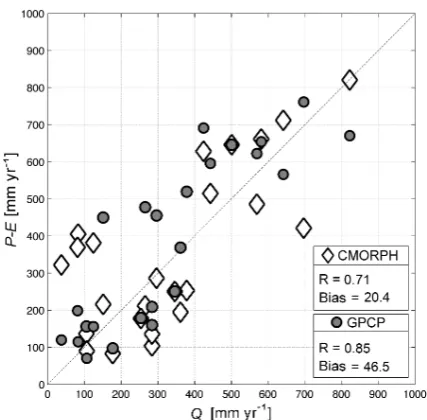
Figure 2 shows the results of the comparison between GLEAM catchment estimates of P−E and river runoff measurements from the 24 rivers for the period 2003– 2006. The figure shows the statistics of the correlation when the methodology is run with CMORPH (R= 0.71, bias = 20.4 mm yr−1) and when it is run with GPCP-1DD (R= 0.85, bias = 46.5 mm yr−1). The higher correlation co-efficient found for the GPCP-basedP−E estimates can be explained by the high positive bias of the CMORPH-based P−E estimates in the rivers of central United States (see Table 1). This is in agreement with the findings of Tian et al. (2007), who reported a clear overestimation of CMORPH rainfall during the warm season in this area. This hypothesis is further analysed in Sect. 4.1.

The correlation in Fig. 2 depends on the validity of three assumptions: (a) the entire volume of river water extracted for human use returns to the river, (b) the catchment is water-tight, and (c) both the lag-time between a rainfall peak in the watershed and the discharge peak in the measuring sta-tion, and the long-term change in soil water storage, can be neglected by considering a relatively long (4 year) period. Moreover, as GLEAM is not a tuned or calibrated hydrolog-ical model, Fig. 2 should be interpreted with a consideration of the magnitude and different origins of the various uncer-tainties. Because river discharge estimates are usually de-rived from a stage-discharge rating curve, they include the er-rors in the measurements of river height and in the discharge data used to calibrate the rating curve, as well as the errors from the interpolation and extrapolation due to changes in river bed roughness, hysteresis effects, etc (see Di Baldas-sarre and Montanari, 2009). On top of those, the volumes of Qare also affected by the uncertainties in the estimation of the discharge-contributing area (given that the observations are presented in mm). On the vertical axes, the uncertainty inP−Eestimates will result from the uncertainty associated with the precipitation product and with GLEAM estimates of land evaporation. The later include the errors in the satellite data used to drive GLEAM (including therefore the uncer-tainties inP as well), the scaling of those to the desired 0.25◦ resolution, and the model structure itself (see Miralles et al., 2011).

Fig. 2. GLEAM estimates ofP−Eare compared to the runoff (Q) from 24 different catchments for the period 2003–2006. Correlation coefficients (R) and mean bias errors (bias) are listed for both the validation exercise using GPCP and the one using CMORPH (gap-filled with GPCP as explained in Sect. 3).

Despite all the possible sources of uncertainty a level of correlation remains as seen in Fig. 2. Furthermore, theP−E estimates are of the right order of magnitude and overall lack a systematic bias relative to the one-to-one line. A global analysis of the spatial distribution ofP−Eestimates is pre-sented in Sect. 4.2; as in previous applications of GLEAM (i.e. Miralles et al., 2010b, 2011), the CMORPH-basedP is chosen for the global run of the methodology. This choice is mainly justified by the better resolution of CMORPH com-pared to GPCP-1DD and the overall better performance of the methodology when CMORPH is applied as reported by the results of the error analyses in Sect. 4.1.

4 Results

4.1 Error analysis

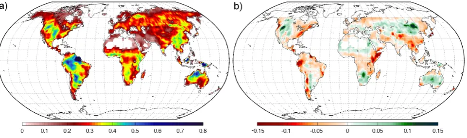
Figure 3a presents the map of the absolute error of GLEAM evaporation anomalies as calculated through Eq. (9) – the RMSE is presented in units of mm day−1_{. The Amazon delta} presents the largest errors, probably because of the large vol-umes of open water and their negative effect on microwave observations. High absolute errors in the rest of Amazonia and south-eastern Asia partly respond to the larger variance of the anomalies in those regions.

Fig. 3. Results of the triple collocation error analyses: (a) absolute error of the evaporation anomalies of GLEAM expressed as RMSE, (b) difference between the RMSE of the evaporation anomalies of GLEAM when it is run with CMORPH and when it is run with

GPCP-1DD (red colour represents the areas where using CMORPH improves the evaporation product). Units are mm day−1.

the high errors of GLEAM in the Great Plains respond to un-certainties in CMORPH, the analysis is repeated using only GPCP-1DD as input of the model. Figure 3b presents the dif-ference between the absolute error of GLEAMEanomalies when the methodology is run with CMORPH and when it is run with GPCP-1DD only (in units of mm day−1). It can be noted that applying GPCP-1DD improves the evaporation es-timates not only over central North America but also around Mongolia, South Africa and the Australian desert. How-ever, Fig. 3b also shows higher quality for the CMORPH-driven evaporation product in the majority (63%) of the do-main common to both precipitation products (60◦N–60◦S). The improvement is significant over the east coast of North America, west coast of South America, Horn of Africa and China. Overall the application of CMORPH leads to better evaporation estimates in all the large regions with complex topography (except for the Rocky Mountains); this finding is in agreement with previous precipitation inter-product com-parisons over complex terrains (e.g. Dinku et al., 2007; Hirpa et al., 2009). This type of information about the spatial dis-tribution of GLEAM errors can be used to selectively pick the inputs that allow a better performance of the model over each region. Notice again that bias errors are not detected by a TC analyses.

The rationale of these three approaches is fundamentally different and the assumption of uncorrelated errors appears therefore justified. However, it may be argued that some de-gree of interdependence exists between the Princeton Uni-versity product and GLEAM due to the relation between the inputs of net radiation in each of the two models. GLEAM uses the NASA/GEWEX Surface Radiation Budget (SRB) net radiation (Stackhouse et al., 2004); the Princeton Univer-sity product is run with the International Satellite Cloud Cli-matology Project (ISCCP) net radiation (Zhang et al., 2004). Like ISCCP net radiation, SRB is also based on ISCCP cloud products. However, SRB net radiation uses different ancil-lary data sources and radiative transfer codes. Both datasets

still present fundamental differences (Zhang et al., 2007; Lin et al., 2008). In addition, the level of agreement between the two is lower at daily timescales (see Troy and Wood, 2009); in this sense the extraction of the seasonally-varying climatology in this exercise will make their errors more un-correlated. Moreover, if this source of dependency was large enough to preclude the TC application, areas in which evap-oration estimates are highly dependent on net radiation (see Sect. 4.2.3 for the global distribution of those areas) would be likely to present lower values of TC-calculated RMSE; this pattern is not indicated by Fig. 3. Finally it is worth mention-ing that this potential dependency would not affect the results presented in Fig. 3b.

4.2 Global application

Table 2. Annual precipitation (P), evaporation (E) and water available for runoff (P−E) divided by continents for the period 2003–2007. The contribution of rainfall interception loss (I) toEis also presented.

Continent P E P−E I

mm mm 103km3 %P mm 103km3 %P mm 103km3 %P

Africa 930 545 16.2 59 385 11.4 41 38 1.1 4 Antarctica 199 21 0.3 11 177 2.5 89 0 0.0 0

Asia 648 388 16.8 60 260 11.3 40 38 1.7 6

Europe 638 369 3.5 58 269 2.6 42 54 0.5 9

N. America 665 413 9.5 62 252 5.8 38 42 1.0 6

Oceania 795 519 4.6 65 276 2.5 35 50 0.4 6

S. America 1712 967 17.0 56 745 13.1 44 144 2.5 8

Total 799 463 67.9 58 336 49.0 42 50 7.2 6

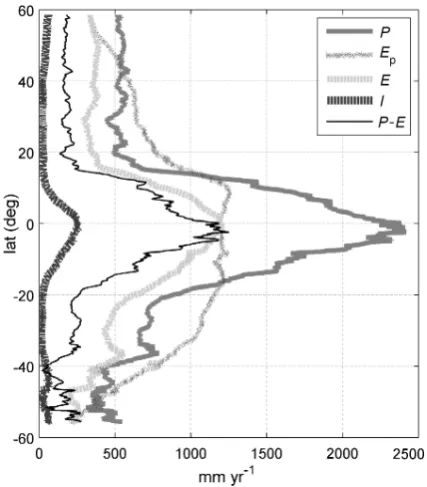
4.2.1 Overview of the global hydrological fluxes For a certain region, and over a sufficiently long period to allow the net change of water storage in the soil to be ne-glected, the land-incoming precipitation is either recycled back into the atmosphere through evaporation, or it drains into the water bodies in the region. Figure 4 presents a graphic overview of the latitudinal partitioning of precip-itation according to GLEAM. Average annual volumes of the different hydrological fluxes are illustrated for the period 2003–2007. All the fluxes are larger close to the Equator due to the higher average incoming radiation, temperature and specific humidity.

Table 2 shows the volumes of total precipitation (P), evap-oration (E– which includes transpiration, soil evaporation, snow sublimation and interception loss) and water avail-able for runoff (P−E) for each continent. The right-hand columns present the contribution of tall vegetation rainfall interception (I) to the long-term partitioning ofP intoEand P−E. The volume of annual global land-surface evapora-tion is estimated as 67.9×103km3. Tall vegetation intercep-tion amounts to 11% of the continental evaporaintercep-tion or 6% of the continental precipitation. Fluxes are larger in South America due to the faster dynamics of the hydrological cy-cle over Amazonia which results from the majority of South America’s land mass being located within the ITCZ; this is more easily recognised when the fluxes are expressed per unit area.

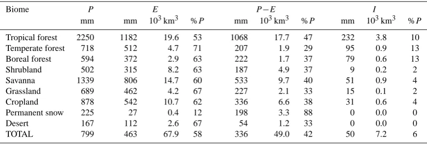
To better understand the role ofI in the partitioning of incoming precipitation over forested ecosystems, the land-use classification scheme of the International Geosphere-Biosphere Programme (IGBP) is used in Table 3 to present the same hydrological fluxes allocated to biome types. Given thatIis calculated for the fraction of tall canopy within each pixel, it can still occur within pixels in which the dominant land use is not forest. Tropical forests contribute to 29% of the global land-surface evaporation and 57% of the global canopy interception loss. In these ecosystems, 20% of the evaporation corresponds to the flux of rainfall interception;

Fig. 4. Magnitude of the different hydrological fluxes as

aver-age along the latitudinal bands (modified from Fisher et al., 2008). The results correspond to the application of GLEAM for the period 2003–2007.Eprefers to potential evaporation.

this flux is equivalent to 22% of the water available for river discharge. At higher latitudes the relative contribution of in-terception loss to land-surface evaporation is also large. In temperate forests, the volume ofI is on average 13% of the incoming precipitation (19% of evaporation).

4.2.2 Spatial distribution of evaporation and its different components

Table 3. Annual precipitation (P), evaporation (E), water available for runoff (P−E) and rainfall interception loss (I) per biome type for 2003–2007.

Biome P E P−E I

mm mm 103km3 %P mm 103km3 %P mm 103km3 %P

Tropical forest 2250 1182 19.6 53 1068 17.7 47 232 3.8 10 Temperate forest 718 512 4.7 71 207 1.9 29 95 0.9 13 Boreal forest 594 372 2.9 63 222 1.7 37 79 0.6 13

Shrubland 502 315 8.2 63 187 4.9 37 9 0.2 2

Savanna 1339 806 14.7 60 533 9.7 40 51 0.9 4

Grassland 689 462 4.2 67 227 2.1 33 15 0.1 2

Cropland 878 542 10.7 62 336 6.6 38 31 0.6 4

Permanent snow 225 27 0.4 12 198 3.3 88 0 0.0 0

Desert 167 112 2.6 67 54 1.2 33 0 0.0 0

TOTAL 799 463 67.9 58 336 49.0 42 50 7.2 6

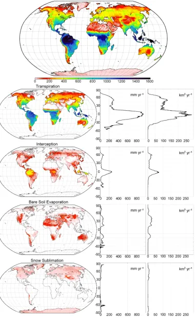
ecosystems. The global distribution of the average annual evaporation during the period 2003–2007 is presented in Fig. 5. The spatial distribution and latitudinal profile for the different components of evaporation is also shown (both in mm yr−1and in km3yr−1). Transpiration contributes to the majority of global land evaporation. It is the largest in the hu-mid tropics due to the sufficient availability of soil moisture during the entire year and the dependency of transpiration on the incoming radiation. Overall, the contribution of canopy interception to the global volume of evaporation is larger than the contribution from bare soil evaporation and snow subli-mation. Evaporation from bare soil is important in desert regions even though it only happens during (and shortly af-ter) the sporadic rainfall events. Peaks of snow sublimation occur in the Himalayas where annual net radiation is higher than in other permanent snow-covered areas due to its loca-tion closer to the Equator.

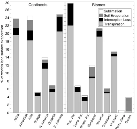
Figure 6 illustrates the contribution to global land-surface evaporation from: (a) each continent, and (b) each biome type. It also shows the relative magnitude of the four con-stituents of the evaporative flux. As seen in Tables 2 and 3, the continent evaporating the largest volume of water is South America (25%), followed by Asia (24.5%) and Africa (23.5%). 29% of world’s evaporation occurs in tropical forests and 21% in savannas. The contribution from tran-spiration amounts to 80% of the total evaporative flux from land; 11% is interception loss, 7% bare soil evaporation and 2% to snow sublimation.

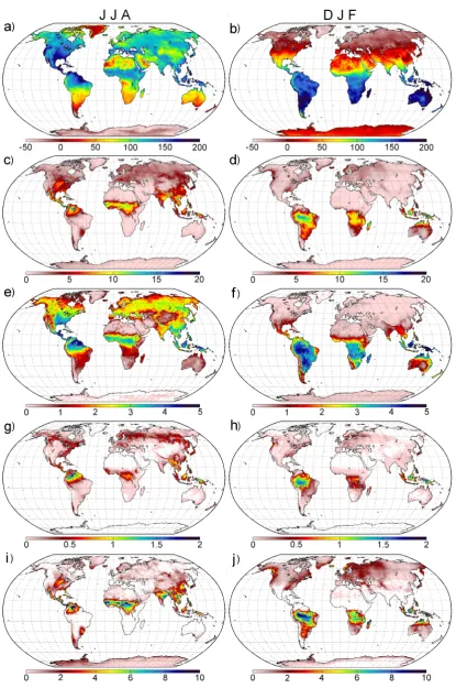
The seasonal distribution of the main inputs and outputs of the methodology is explored in Fig. 7. Global maps ofRn,P, E,I andP−Efor 2003–2007 are presented as an average for two different periods: the months of June, July and Au-gust (JJA), and December, January and February (DJF). The global distributions of bothI andP−E are dominated by the seasonal cycle ofP. The observed patterns also indicate the lower importance of seasonal changes inE– compared to changes inP – in the availability of water for runoff at

different times of the year. The seasonal distribution ofEis mainly dominated by the cycle ofRnover most of the world

(see also Sect. 4.2.2). The largest seasonal variations inE are found in subtropical areas with sufficient input ofP dur-ing the summer period; in some of these regions the volume of Ein summer-time becomes almost one order of magni-tude larger than during winter-time (see for instance North-ern Australia, SouthNorth-ern Africa or the east coast of United States). In desert regions where rainfall events rarely happen (like central Australia or the Arabian Peninsula) the volumes of evaporation remain low during the entire year and the sea-sonal distribution ofEis independent of the cycle ofRn.

4.2.3 Drivers of evaporation

The main factors that limit land evaporation are the available energy and the volume of precipitation. The spatial and tem-poral distribution of these limiting factors, and the strength of the correlation of evaporation with one particular driver, can provide valuable information on the seasonal dynamics of evaporation in a particular area. Teuling et al. (2009) hy-pothesised that regional trends in land evaporation respond to trends in the limiting drivers. Only when we know to what extent a specific driver is controlling the evaporation process, known changes in that controlling factor may be translated into long-term changes in evaporation.

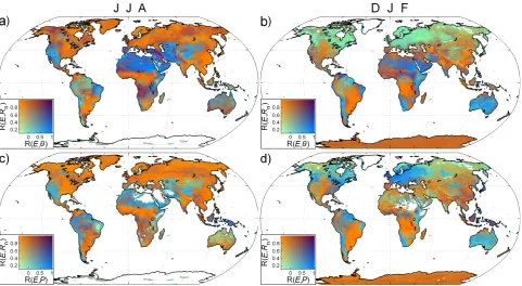
Here, the GLEAM-estimated relationship between land evaporation and its external drivers is analysed at a global scale. Figure 8 gives a global overview of such analysis for the period 2003–2007. This figure has been made using the technique by Teuling et al. (2010) for plots with bivariate colour maps. Figure 8a shows for JJA the global distribution of the correlation coefficient between daily time series ofE andRnand the correlation coefficient betweenEandθ

Fig. 5. Decomposition of 2003–2007 average annual evaporation (mm) into its contributing fluxes. The latitudinal profiles are shown in units

Fig. 6. Contribution to global land-surface evaporation (in %) for

each: (a) continent, and (b) biome type. The relative contribution of the constituents of evaporation is presented separately.

present the global distribution of the correlation betweenE andRn, andEandP for JJA and DJF, respectively.

The model predicts that most of the JJA daily variability of Eover Central Europe and North America can be explained by the dynamics inRn(see high correlation betweenEand Rnin Fig. 8a). In forested areas in boreal winter-timeP

be-comes important (see Fig. 8d) and the relation with Rn is

weaker. Despite the high correlation betweenE andP, E remains relatively uncorrelated withθ; this suggests that the soil remains under no stress for transpiration. The compo-nent of forest evaporation that is affected byP (and govern-ing the dynamics ofE) is therefore not the transpiration flux but the rainfall interception loss. For tropical rain forests, despite the fact thatRn remains in general the largest

con-trolling factor,P is also identified as an important driver of evaporation in both seasons.

Areas presenting high correlations betweenEandθ cor-respond mainly to arid and semi-arid regions, and especially during summer-time (see Fig. 8a and b). In these regions the correlation ofEwith the time series ofP is lower than the correlation betweenE andθ; this is because soil moisture is a more direct indicator of plant water stress. The areas where soil moisture is likely to limit the evaporative flux can also be seen in Fig. 9. This figure presents the global aver-age (2003–2007) distribution of the estimates of daily stress factor,S– which equals (E−I)/Ep(see Sect. 2.1). The left

map represents the months of JJA; the right map shows DJF. GLEAM calculatesS at daily time-step based on estimates of soil moisture and vegetation optical depth (see Miralles et al., 2011). Values ofS= 1 correspond to areas where there is

sufficient water to meet the atmospheric evaporative demand; values ofS= 1 are present in areas where the shortage of wa-ter restricts the actual rate of evaporation under its potential value. It can be seen that over the majority of the world’s land surface, land conditions regulate to certain extent the flux of evaporation. In high latitudes the availability of wa-ter is generally sufficient to meet the atmospheric demand. Arid and semi-arid regions, however, remain under evapora-tive stress during almost the entire year. The seasonal spatial patterns ofSare strongly related to the seasonal distribution of P (Fig. 7c and d) and the distribution of the correlation betweenEandθ(Fig. 8a and b).

5 Discussion

The average annual land-surface evaporation estimated by GLEAM for the period 2003–2007 is 67.9×103km3. This number is comparable to other estimates of average an-nual land evaporation – e.g. the 71×103km3 found by Baumgartner and Reichel (1975) (see Dolman and Gash, 2010), the 65.5×103km3found by Oki and Kanae (2006), the 65×103km3 reported by Jung et al. (2010) or the 65.8×103km3by Schlosser and Gao (2010). Lim and Rod-erick (2009) analysed the global partitioning of precipitation over land making use of the GCMs from the Intergovern-mental Panel on Climate Change (IPCC) Fourth Assessment Report (AR4). Despite referring to a different period than the one presented here (2003–2007 versus 1970–1999) the volume of incoming precipitation is similar in both stud-ies. While the ensemble of GCMs estimated that 70% of the global land precipitation was evaporated and 30% was avail-able for runoff (P−E), the global partitioning in GLEAM is somewhat different: 58% evaporation and 42% water avail-able for runoff. Despite this difference the relative contri-bution from each continent to global E and global P−E agrees well in both studies. One exception is South America in which the GCMs estimated 51% lessP−Ethan GLEAM. It is worth mentioning that this dissimilarity responds mainly to the different volumes of precipitation and not of evapora-tion.

Fig. 7. Average fluxes for the period 2003–2007 separately presented for JJA (left panel) and DJF (right panel): (a) and (b) show the

Fig. 8. The upper panel shows the estimated correlation (R) of daily time series ofEwithRnandθfor (a) JJA and (b) DJF. The bottom figures show the correlation of dailyEwithRnandP during (c) JJA and (d) DJF. All the results correspond to the period 2003–2007.

Fig. 9. Estimated stress factor (S) as averaged for the months of JJA and DJF

this uncertainty and enhances the reliability of GLEAM es-timates ofEandP−Ein areas of sparse observations like Africa.

Fisher et al. (2008) obtained similar results (both in abso-lute and in relative terms) to the ones presented in the latitu-dinal profile of annual fluxes shown in Fig. 4. Humid tropics show a value of land evaporation around 50% of the incom-ing precipitation, in accordance with the level of rainfall re-cycling in these areas reported by Salati and Vose (1984). This latitudinal profile is in agreement with the hypothesis that at high latitudes in winter-time, the flux of intercep-tion loss – dominated by the aerodynamic forces rather than

the Penman-Monteith equation, the aerodynamic term (and not the energy one) is responsible for the major part of the flux. This is the main reason why interception loss requires a separate estimation, and why PT energy-based approaches are not suitable for its estimation.

Traditionally, studies on evaporation drivers have been fo-cused on net radiation and soil moisture (considered only as the link between precipitation and evaporation). However, an important component of the evaporative flux from forests, canopy-intercepted rainfall, will not be directly affected by the soil moisture dynamics. Moreover, as stated above, the flux of evaporated water from wet canopies is relatively in-dependent from the net radiation. Teuling et al. (2009) anal-ysed in detail the drivers of the evaporative flux over Eu-rope and North America focusing on net radiation and pre-cipitation, but considering the latter only as a surrogate for soil moisture. Their results were extensively validated us-ing FLUXNET data but rain-days were not included in this validation and therefore the role of interception could not be identified. The daily frequency and separate estimation of interception within GLEAM allows a detailed study of these interactions. However, while Teuling et al. (2009) compared independent estimates, in the study presented in Sect. 4.2.3 the estimates ofEare dependent on the values ofP,Rnand θ, and therefore the results rely on the sensitivity of GLEAM Eto these variables. Consequently this study merely aims to understand how GLEAM reproduces interactions between land and atmosphere and how it estimates the relative im-portance of the evaporation drivers in different regions in the world.

Figure 8a and c shows how in summer-time and over Cen-tral Europe and North America, most of the variability of daily GLEAM estimates ofE can be explained by the dy-namics in Rn. This is in agreement with Fig. 7a,b,e,f that

illustrate how in the majority of the world’s land surface the seasonality ofE follows closely the seasonality of the in-coming solar energy. However, in forested regions and dur-ing winter-time the relationship is not obvious (see Fig. 8b). This low dependency between the time series ofEand the time series ofRnis a response to the higher relative

impor-tance ofIas a component ofE. This happens because of the low volumes of transpiration in winter-time. As can be ap-preciated from Fig. 8d, in forested regions under conditions of low incoming radiation, the model identifies the availabil-ity of water on the canopy (dominated by the volume ofP and its duration) as an important factor determining the dy-namics of evaporation. The low correlations found withθ over the same areas, suggest that the correlation withP is not a response to conditions of soil water deficit.

Trends in soil moisture can be responsible for the long-term changes in land evaporation; this happens over regions where water availability is the main control on the evapora-tion (see Teuling et al., 2009). Jung et al. (2010) analysed the results of their FLUXNET data-based approach (Jung et al., 2009) to reveal a positive trend in global land-surface

evaporation from 1982 to 1997; from 1998 this trend slowed down, attributed to the decrease in soil moisture over the Southern Hemisphere. Dark blue-coloured regions in Fig. 8a and b represent the areas where GLEAM identifies that a long-term decrease in soil moisture could potentially induce a negative trend in land evaporation. They are mainly arid and semi-arid regions, where the rate of actual evaporation rarely matches the potential rate (especially during summer-time) and it is the availability of water in the soil that will determine the volume of daily evaporation (see also Fig. 9). This dependency on the soil moisture underlines the impor-tance of correctly parameterising the soil water content and the stress conditions for those areas.

6 Conclusions

Large differences in the estimates of land-surface evapora-tion from the currently existing methodologies (Jim´enez et al., 2011; M¨uller et al., 2011) indicate that land evaporation remains one of the most uncertain terms in the global water cycle. GLEAM is a new alternative to estimate global evap-oration and its different components by combining satellite-observable variables within a simple bio-physical approach. It aims to fill the gaps from previous satellite-based evapo-ration models acknowledging the importance of estimating interception loss through a widely-tested model (Gash’s an-alytical model), and moderating PT estimates of latent heat flux by considering the soil water stress conditions over the entire root-zone. As with every model, GLEAM is a simpli-fication of reality: results presented here are affected by the assumptions taken in the parameterisation of the bio-physical processes within the methodology. However, the constituent parts of GLEAM have been successfully validated by com-parison with in situ data over different ecosystems and the error structure of the estimates has been analysed in detail; this sets the level of credibility of the results presented in this paper.

Ongoing activities include the application of GLEAM to develop a 24 year database (from 1984 to 2007), and an inter-product comparison with existing global fields of evaporation within the LandFlux-EVAL initiative of the GEWEX Radi-ation Panel (Jim´enez et al., 2011; M¨uller et al., 2011). The applicability of triple collocation will be further explored us-ing the longer record of evaporation; different sources of evaporation will be applied to test the sensitivity of the es-timated errors to the potential dependency between GLEAM and Princeton University products. The dataset could ad-ditionally be used to investigate trends in land evaporation and their relation to ocean oscillations, the effects of land-use changes such as desertification or deforestation on the hydrological cycle, and the coupling between land and atmo-spheric processes.

All GLEAM products will become freely available through the web portal hosted at the VU University Ams-terdam Geo-services website (http://geoservices.falw.vu.nl). Acknowledgement. The work was undertaken as part of the European Union (FP6) funded Integrated Project called WATCH (Contract No. 036946). The data used in the validation of theP−E

estimates was provided by the Global Runoff Data Centre, 56068 Koblenz, Germany. We would like to thank A. J. Teuling for his feedback on the application of the technique explained in Teuling et al. (2010) and his valuable comments. We also thank C. Jim´enez for his detailed review, and R. H. Reichle and J. Sheffield for providing the datasets used in the triple collocation study.

Edited by: B. van den Hurk

References

Baumgartner, A. and Reichel, E.: The World Water Balance: Mean Annual Global Continental and Maritime Precipitation, Evapo-ration and Runoff, Elsevier Scientific Publishing Company, Am-sterdam, The Netherlands, Oxford, UK and New York, USA, 1975.

Blyth, E. M., Shuttleworth, W. J, and Harding, R. J.: Summary of the GEWEX International Symposium on Global Land-surface Evaporation and Climate, Hydrol. Process., 23, 3411–3412, 2009.

Bosilovich, M.: NASA’s Modern Era Retrospective-analysis for Re-search and Applications: Integrating Earth Observations, Earth-Zine, E-Zine article, 2008.

Choudhury, B. J. and DiGirolamo, N. E.: A biophysical process-based estimate of global land surface evaporation using satellite and ancillary data; I. Model description and comparison with ob-servations, J. Hydrol., 205, 164–185, 1998.

De Jeu, R. A. M., Wagner, W., Holmes, T. R. H., Dolman, A. J., van de Giesen, N. C., and Friesen, J.: Global soil moisture patterns observed by space borne microwave radiometers and scatterom-eters, Surv. Geophys., 29, 399–420, 2008.

Di Baldassarre, G. and Montanari, A.: Uncertainty in river dis-charge observations: a quantitative analysis, Hydrol. Earth Syst. Sci., 13, 913–921, doi:10.5194/hess-13-913-2009, 2009. Dinku, T., Ceccato, P., Grover-Kopec, E., Lemma, M., Connor, S. J.,

and Ropelewski, C. F.: Validation of satellite rainfall products

over East Africa’s complex topography, Int. J. Remote Sens., 28, 1503–1526, doi:10.1080/01431160600954688, 2007.

Dirmeyer, P. A., Gao, X. A., Zhao, M., Guo, Z. C., Oki, T., and Hanasaki, N.: GSWP-2 Multimodel anlysis and implications for our perception of the land surface, B. Am. Meteorol. Soc., 87, 1381–1397, 2006.

Dolman, A. J. and De Jeu, R. A. M.: Evaporation in focus, Nat. Geosci., 3, 296, 2010.

Dolman, A. J. and Gash, J. H.: Evaporation in the global hydrolog-ical cycle, in: Treatise on Water Science, edited by: Wilderer, P., Treatise on Water Science, vol. 2, Academic Press, Oxford, 79-87, 2010.

Dorigo, W. A., Scipal, K., Parinussa, R. M., Liu, Y. Y., Wagner, W., de Jeu, R. A. M., and Naeimi, V.: Error characterisation of global active and passive microwave soil moisture datasets, Hydrol. Earth Syst. Sci., 14, 2605–2616, doi:10.5194/hess-14-2605-2010, 2010.

Ebert, E. E., Janowiak, J. E., and Kidd, C.: Comparison of near-real time precipitation estimates from satellite observations and numerical models, B. Am. Meteorol. Soc., 88, 47–64, 2007. Fisher, J. B., Tu, K. P., and Baldocchi, D. D.: Global estimates of

the land-atmosphere water flux based on monthly AVHRR and ISLSCP-II data, validated at 16 FLUXNET sites, Remote Sens. Environ., 112, 901–919, 2008.

Gash, J. H.: An analytical model of rainfall interception by forests, Q. J. Roy. Meteorol. Soc., 105, 43–55, 1979.

Gash, J. H. and Shuttleworth, W. J.: Vegetation controls on evapora-tion – commentary, in: Benchmark Papers in Hydrology: Evap-oration, edited by: Gash, J. H. and Shuttleworth, W. J., IAHS Press, Wallingford, 233–239, 2007.

Hirpa, F. A., Gebremichael, M., and Hopson, T.: Evaluation of high resolution satellite precipitation products over very com-plex terrain in Ethiopia, J. Appl. Meteorol. Clim., 49, 1044-1051, doi:10.1175/2009JAMC2298.1, 2009.

Huffman, G. J., Adler, R. F., Morrissey, M. M., Bolvin, D. T., Cur-tis, S., Joyce, R., McGavock, B., and Susskind, J.: Global pre-cipitation at one-degree daily resolution from multisatellite ob-servations, J. Hydrometeorol., 2, 36–50, 2001.

Jim´enez, C., Prigent, C., and Aires, F.: Toward an esti-mation of global land surface heat fluxes from multisatel-lite observations, J. Geophys. Res.-Atmos., 114, D06305, doi:10.1029/2008JD011392, 2009.

Jim´enez, C., Prigent, C., M¨uller, B., Seneviratne, S. I., Mc-Cabe, M. F., Wood, E. F., Rossow, W. B., Balsamo, G., Betts, A. K., Dirmeyer, P. A., Fisher, J. B., Jung, M., Kanamitsu, M., Reichle, R. H., Reichstein, M., Rodell, M., Sheffield, J., Ku, T., and Wang, K.: Global inter-comparison of 12 land surface heat flux estimates, J. Geophys. Res.-Atmos., 116, D02102, doi:10.1029/2010JD014545, 2011.

Joyce, R. J., Janowiak, J. E., Arkin, P. A., and Xie, P.: CMORPH: A method that produces global precipitation estimates from pas-sive microwave and infrared data at high spatial and temporal resolution, J. Hydrometeorol., 5, 487–503, 2004.

Jung, M., Reichstein, M., Ciais, P., Seneviratne, S., Sheffield, J., Goulden, M., Bonan, G., Cescatti, A., Chen, J., de Jeu, R., Dolman, A. J., Eugster, W., Gerten, D., Gianelle, D., Go-bron, N., Heinke, J., Kimball, J., Law, B., Montagnani, L., Mu, Q., Mueller, B., Oleson, K., Papale, D., Richardson, A., Roupsard, O., Running, S., Tomelleri, E., Viovy, N., We-ber, U., Williams, C., Wood, E., Zaehle, S., and Zhang, K.: Recent decline in the global land evapotranspiration trend due to limited moisture supply, Nature, 467, 951–954, doi:10.1038/nature09396, 2010.

Lim, W. H. and Roderick, M. L.: An Atlas of the Global Water Cycle: Based on the IPCC AR4 models, ANU E Press, Canberra, 2009.

Lin, B., Stackhouse Jr., P. W., Minnis, P., Wielicki, B. A., Hu, Y., Sun, W., Fan, T.-F., and Hinkelman, L. M.: Assessment of global annual atmospheric energy balance from satellite observations, J. Geophys. Res., 113, D16114, doi:10.1029/2008JD009869, 2008. Love, T. B., Kumar, V., Xie, P. and Thiaw, W.: A 20-year daily Africa precipitation climatology using satellite and gauge data. In Proceedings of the 84th AMS Annual Meeting, P5.4. Conference on Applied Climatology, Seattle, WA, 2004.

Miralles, D. G., Crow, W. T., and Cosh, M. H.: Estimating spatial sampling errors in coarse-scale soil moisture estimates derived from point-scale observations, J. Hydrometeorol., 11, 1423– 1429, doi:10.1175/2010JHM1285.1, 2010a.

Miralles, D. G., Gash, J. H., Holmes, T. R. H., De Jeu, R. A. M., and Dolman, A. J.: Global canopy interception from satel-lite observations, J. Geophys. Res.-Atmos., 115, D16122, doi:10.1029/2009JD013530, 2010b.

Miralles, D. G., Holmes, T. R. H., De Jeu, R. A. M., Gash, J. H., Meesters, A. G. C. A., and Dolman, A. J.: Global land-surface evaporation estimated from satellite-based observations, Hydrol. Earth Syst. Sci., 15, 453–469, doi:10.5194/hess-15-453-2011, 2011.

Mu, Q., Heinsch, F. A., Zhao, M., and Running, S. W.: Develop-ment of a global evapotranspiration algorithm based on MODIS and global meteorology data, Remote Sens. Environ., 111, 519– 536, 2007.

M¨uller, B., Seneviratne, S. I., Jim´enez, C., Corti, T., Hirschi, M., Balsamo, G., Ciais, P., Dirmeyer, P., Fisher, J. B., Guo, Z., Jung, M., Maignan, F., McCabe, M. F., Reichle, R., Reichstein, M., Rodell, M., Sheffield, J., Teuling, A. J., Wang, K., Wood, E. F., and Zhang, Y.: Evaluation of global observations-based evapo-transpiration datasets and IPCC AR4 simulations, Geophys. Res. Lett., doi:10.1029/2010GL046230, in press, 2011.

Murphy, D. M. and Koop, T.: Review of the vapour pressures of ice and supercooled water for atmospheric applications, Q. J. Roy. Meteorol. Soc., 131, 1539–1565, 2005.

Oki, T. and Kanae, S: Global hydrological cycles and world water resources, Science, 313, 1068-1072, 2006.

Peixoto, J. P. and Oort, A. H.: Physics of Climate, American Insti-tute of Physics, New York, USA, 172 pp., 1992.

Salati, E. and Vose, P. B.: Amazon Basin: a system in equilibrium, Science, 225, 129–138, 1984.

Schlosser, C. A. and Gao, X.: Assessing evapotranspi-ration estimates from the second Global Soil Wetness Project (GSWP-2) simulations, J. Hydrometeor, 11, 880-897, doi:10.1175/2010JHM1203.1, 2010.

Scipal, K., Holmes, T., de Jeu, R., Naeimi, V., and Wagner, W.: A possible solution for the problem of estimating the error struc-ture of global soil moisstruc-ture data sets, Geophys. Res. Lett., 35, L24403, doi:10.1029/2008gl035599, 2008.

Sellers W. D.: Physical Climatology, University of Chicago Press, Chicago, IL, USA, 1965.

Sheffield, J., Wood, E. F., and Munoz-Arriola, F.: Long-term regional estimates of evapotranspiration for Mexico based on downscaled ISCCP data, J. Hydrometeorol., 11, 253–275, 2010. Shuttleworth, W. J. and Calder, I. R.: Has the Priestley-Taylor equa-tion any relevance to forest evaporaequa-tion?, J. Appl. Meteorol., 18, 639–646, 1979.

Stackhouse, P. W., Gupta, S. K., Cox, S. J., Mikovitz, J. C., Zhang, T., and Chiacchio ,M.: 12 year surface radiation budget data set GEWEX News, 14, 2004.

Stewart, J. B: Evaporation from the wet canopy of a pine forest, Water Resour. Res., 13, 915–921, 1977.

Stoffelen, A.: Toward the true near-surface wind speed: Error mod-eling and calibration using triple collocation, J. Geophys. Res., 103, 7755-7766, doi:10.1029/97jc03180, 1998.

Teuling, A. J., Hirschi, M., Ohmura, A., Wild, M., Reichstein, M., Ciais, P., Buchmann, N., Ammann, C., Montagnani, L., Richard-son, A. D., Wohlfahrt, G., and Seneviratne, S. I.: A regional perspective on trends in continental evaporation, Geophys. Res. Lett., 36, L02404, doi:10.1029/2008GL036584, 2009.

Teuling, A. J., St¨ockli, R., and Seneviratne, S. I.: Bivariate colour maps for visualizing climate data (short communication), Int. J. Climatol., doi:10.1002/joc.2153, in press, 2010.

Tian, Y., Peters-Lidard, C. D., Chaudhury, B. J., and Garcia, M.: Multitemporal analysis of TRMM-based satellite precipitation products for land data assimilation applications, J. Hydromete-orol., 8, 1165–1183, 2007.

Troy, T. J. and Wood, E. F.: Comparison and evaluation of gridded radiation products across northern Eurasia, Environ. Res. Lett., 4, 045008, doi:10.1088/1748-9326/4/4/045008, 2009.

Valente, F., David, J. S., and Gash, J. H.: Modelling interception loss for two sparse eucalypt and pine forests in Central Portugal using reformulated Rutter and Gash analytical models, J. Hy-drol., 190, 141–162, 1997.

Zeweldi, D. A. and Gebremichael, M.: Evaluation of CMORPH precipitation products at fine space-time scales, J. Hydrometeo-rol., 10, 300–308, 2009.

Zhang, K., Kimball, J. S., Nemani, R. R., and Running, S. W.: A continuous satellite-derived global record of land surface evapotranspiration from 1983 to 2006, Water Resour. Res., 46, W09522, doi:10.1029/2009WR008800, 2010.

Zhang, Y., Rossow, W. B., Lacis, A. A., Oinas, V. and Mishchenko, M. I.: Calculation of radiative fluxes from the surface to top of atmosphere based on ISCCP and other global data sets: Refinements of the radiative transfer model and the input data, J. Geophys. Res., 109, D19105, doi:10.1029/2003JD004457, 2004.