www.hydrol-earth-syst-sci.net/12/943/2008/ © Author(s) 2008. This work is distributed under the Creative Commons Attribution 3.0 License.
Earth System
Sciences
Comparing model performance of two rainfall-runoff models in the
Rhine basin using different atmospheric forcing data sets
A. H. te Linde1,2, J. C. J. H. Aerts1, R. T. W. L. Hurkmans3, and M. Eberle4
1Institute for Environmental Studies (IVM), Faculty of Earth and Life Sciences, Vrije Universiteit, De Boelelaan 1087, 1081
HV Amsterdam, The Netherlands
2Deltares, Rotterdamseweg 185, 2629 HD Delft, The Netherlands
3Hydrology and Quantitative Water Management, Wageningen University, Droevendaalsesteeg 4,
6708 PB Wageningen, The Netherlands
4Federal Institute of Hydrology (BfG), Am Mainzer Tor 1, D-56068 Koblenz, Germany
Received: 16 November 2007 – Published in Hydrol. Earth Syst. Sci. Discuss.: 4 December 2007 Revised: 19 March 2008 – Accepted: 22 May 2008 – Published: 25 June 2008
Abstract. Due to the growing wish and necessity to simu-late the possible effects of climate change on the discharge regime on large rivers such as the Rhine in Europe, there is a need for well performing hydrological models that can be applied in climate change scenario studies. There exists large variety in available models and there is an ongoing debate in research on rainfall-runoff modelling on whether or not phys-ically based distributed models better represent observed dis-charges than conceptual lumped model approaches do. In ad-dition, it is argued that Land Surface Models (LSMs) carry the potential to accurately estimate hydrological partitioning, because they solve the coupled water and energy balance. In this paper, the hydrological models HBV and VIC were com-pared for the Rhine basin by testing their performance in sim-ulating discharge. Overall, the semi-distributed conceptual HBV model performed much better than the distributed land surface model VIC (E=0.62,r2=0.65 vs.E=0.31,r2=0.54 at Lobith). It is argued here that even for a well-documented river basin such as the Rhine, more complex modelling does not automatically lead to better results. Moreover, it is con-cluded that meteorological forcing data has a considerable influence on model performance, irrespectively to the type of model structure and the need for ground-based meteoro-logical measurements is emphasized.
Correspondence to: A. H. te Linde
1 Introduction
The semi-distributed conceptual model HBV (Hydrol-ogiska Byr˚ans Vattenbalansavdelning) (Bergstr¨om, 1976; Lindstr¨om et al., 1997) has been applied in multiple studies for the Rhine basin since 1999 by both the German Federal Institute of Hydrology and the Dutch Ministry of Transport, Public Works and Water Management (M¨ulders et al., 1999; Weerts and Van der Klis, 2004; Eberle et al., 2005). How-ever, the HBV model does not exactly describe all the phys-ical processes that are believed to be of major importance for the simulation of timing and magnitude of extreme flood and drought events (Sch¨ar, 1998; Ward and Robinson, 2000). Potential evaporation, for example, is calculated using the Penman-Wendling approach based on temperature and sun-shine duration (Eberle et al., 2005) while more innovative methods are available using coupled water and energy bal-ance simulations. Recently the state of the art distributed land surface model (LSM) VIC (Variable Infiltration Capac-ity) (Liang et al., 1994) has been applied on the Rhine basin (Hurkmans et al., 2008), which does describe all relevant land surface processes, including the energy balance, and therefore carries the potential to estimate hydrological parti-tioning more accurately than the HBV model does. Because of a realistic representation of evaporation processes in land surface models such as done within VIC, Troy et al. (2007) argue that these types of models are inevitable when perform-ing climate and land use change scenario studies.
However, the application of a distributed land surface model such as VIC at a macro-scale river basin, such as the Rhine basin, is still a highly simplified representation because of its spatial resolution. Even when using a very fine grid, in the order of tens or hundreds of meters and by that sabotaging calculation time, it will never represent ac-tual processes that vary at a scale of trees and ditches (Uh-lenbrook, 2003) and the actual heterogeneity of hydrological processes. Considering the required input data and computer capacity, the question remains whether more complex and demanding models such as VIC can be preferred over sim-pler, conceptual water balance models such as HBV. A better understanding of the use and capacity of different hydrolog-ical models would enhance the confidence in future climate scenario studies using these hydrological models. An un-certainty analysis of all processing steps from climate sce-narios via downscaling methods to hydrological modelling is required. Estimating uncertainty of model simulations starts with analysing model performance using historical data. In this view, the goal of this paper is to compare the hydrolog-ical models HBV and VIC by testing their performance for simulating historical discharge. Based on the performance of both models, a recommendation can be made for the type of hydrological model to be preferred for climate change sce-nario studies.
Since both models have a different physical structure re-sulting from a different theoretical background, the divergent concepts in rainfall-runoff modelling are first addressed in Sect. 2. In Sect. 3, the models and study area are described.
In Sect. 4, the methods that are used for comparing atmo-spheric forcing data and model performance are explained, whereupon the results are presented in Sect. 5. Finally, the results are discussed and several conclusions are drawn in Sect. 6.
2 Divergent concepts in rainfall-runoff modelling
On the other hand, some researchers advocate a more straightforward hydrologic approach claiming that more complex modelling does not always lead to better results. Depending on dominant processes, data availability, scale and application of the model, one should select the appro-priate modelling approach which can result in using a very simple model (Booij, 2003; Seibert, 1999). When formu-lating their famous and widely used performance criterion, Nash and Sutcliffe (1970) already warned for the risk of over-parameterized models. In recent years, the debate on model complexity versus model performance has intensified again and Beven (2001, 2002a, b) goes a step further and critically analyzed the constraints of distributed modelling. The perfect hydrological model that represents reality accu-rately will never exist, as there will always remain necessary approximations of processes and parameters at the model el-ement scale. Beven (2001) claims that the ongoing pursue to a realistic representation has led to unjustified determin-ism in many distributed modelling applications and a lack of recognition of the problems of distributed modelling such as nonlinearity, scale and equifinality (which arises when many different parameter sets give equally good results). Further-more, Savenije (2001) states that the large number of pa-rameters in distributed models make it possible to repre-sent hydrological behaviour well for the current situation, but due to over-parameterization these models are not the right tools to describe what will happen if certain charac-teristics of the basin change, such as land use or soil char-acteristics. Savenije (2001) suggests to further develop a new data-based top down approach (Jothityangkoon et al., 2001) in which relatively simple basin response functions describe complex hydrological processes at scales with suf-ficient level of aggregation. It consists of beginning with a large time step and gradually introducing the complexity re-quired to meet the needs of shorter time steps. This resem-bles the conceptual approach of already long-existing water balance models like Sacramento, HBV and RhineFlow (Van Deursen and Kwadijk, 1993). Bogaard (2005) argues that the main challenges in understanding discharge generating pro-cesses appear to be related to the scale of the propro-cesses. Mi-cro scale hydrological processes are highly heterogeneous, non-linear and interconnected, with the consequence that up-scaling from micro- to basin scale and subsequent parameter-ization is practically impossible. In conclusion, hydrologists are looking for answers to match the observed complexity at the plot-scale, with the apparent simplicity that arises at the basin scale. Comparing the HBV and VIC models, having opposed model structures, for their performance in a well-documented river basin like the Rhine basin, will add to the debate on divergent concepts in hydrological modelling.
3 Model description and study area
3.1 VIC
The Variable Infiltration Capacity (VIC) model (Liang and Zhenghui, 2001; Liang et al., 1994) is a distributed, macro-scale land surface model with a physically based soil-vegetation-atmosphere transfer scheme (SVATS), which solves both the water and energy balance. It is distinguished from other SVATS by its focus on runoff processes. These are represented through the variable infiltration curve, a pa-rameterization of the effects of sub-grid variability in soil moisture holding capacity, from which the model takes its name, and a representation of non-linear baseflow. Rout-ing of surface runoff and baseflow is done by the algorithm developed by Lohmann et al. (1996). A more extensive description of the modelling scheme is available in Hurk-mans (2008), who recently developed the VIC model for the Rhine basin at a spatial resolution of 0.05×0.05 degree. The seven required atmospheric input time series are derived from a re-analysis dataset and are described in Sect. 4.1. 3.2 HBV
The HBV-96 model (Hydrologiska Byr˚ans Vattenbal-ansavdelning) (Bergstr¨om, 1976; Lindstr¨om et al., 1997) model is a semi-distributed conceptual model. The model that is used in this study simulates discharge on a daily basis for 134 sub-basins of the Rhine. The model simu-lates snow accumulation, snowmelt, actual evapotranspira-tion, soil moisture storage, groundwater depth and runoff. The required forcing data are precipitation, temperature, and potential evaporation. The model consists of different rou-tines in which snowmelt is computed by a day-degree rela-tion, and groundwater recharge and actual evaporation are functions of actual water storage in a soil box. Discharge formation is represented by a linear reservoir for base flow and a non-linear approach for fast runoff components. The sub-basins are linked together with a simplified Muskingum approach (Shaw, 2002) to simulate routing processes. The HBV model was developed for the Rhine in several steps since 1997 by the Dutch Institute for Inland Water Manage-ment and Waste Water TreatManage-ment (RIZA) and the German Federal Institute of Hydrology (BfG). A complete descrip-tion of the HBV calculadescrip-tion scheme and the model structure for the Rhine basin is found in Eberle et al. (2005).
3.3 Rhine basin
Fig. 1. Map of the Rhine basin showing (a) 134 HBV sub-catchments; (b) the calculation grid used in VIC (0.05×0.05 degree); and (c) discharge measurement locations and sub-basins used in the analysis.
cover in the Alps is characterized by agricultural land in the lower regions and by forest, shrubs, meadows, unvegetated areas and glaciers on the higher slopes. The area of the Upper Rhine between Basel and Bingen is hilly, with eleva-tions reaching over 1000 m a.s.l., but with flood plains along the main rivers. In the flood plains there is urban develop-ment, while the hills are mainly forested. The main tribu-taries Neckar, Main, Moselle, Lahn and Sieg have a mixed land use pattern, with agriculture and vineyards on the val-ley slopes, and forest on the hillslopes and mountains. The Middle Rhine has incised in higher grounds, which resulted in a deep narrow valley without floodplains. The relatively flat and low-lying Lower Rhine area downstream of Cologne until the Dutch-German border is an urbanized area with a
considera-tion in the present study vary from 5304 km2to 27 142 km2, as can be seen from Table 1 among other basin characteris-tics.
4 Methods
4.1 Data
Both the HBV and VIC models were forced using down-scaled ECMWF ERA15 atmospheric re-analysis data, which is provided by the Max Planck Institute for Meteorology (MPI), Hamburg, Germany. The regional climate model REMO (Jacob, 2001) was used for downscaling and this dataset will be further referred to as ERA15. The ERA15 data set comprises the years 1993 through 2003, at a 3-hourly time step, with a grid resolution of 0.088 degrees and pro-vides the following forcing data: precipitation, temperature, specific humidity, air pressure, downward radiation (short-wave and long(short-wave) and windspeed. These input data are all required to run the VIC model.
To compare this data to observations, two additional me-teorological datasets are available. First, a historical data set is available from the International Commission for the Hydrology of the Rhine basin (CHR). This data set is re-ferred to as CHR and contains daily values of precipitation and temperature for the years 1961 through 1995, which are based on 36 measurement stations throughout the basin (Sprokkereef, 2001). Second, a historical dataset using in-terpolated measured data is available from the Climate Re-search Unit (CRU) where they develop a number of global datasets widely used in climatic research. This data set is referred to as CRU (Mitchell and Jones, 2005) and contains precipitation and temperature values at a monthly time step and comprises the years 1900 through 1998, with a grid res-olution of 0.5 degrees.
HBV was also forced by CHR precipitation and tempera-ture data and VIC only by CHR precipitation. VIC could not be forced by CHR temperature, because the models needs daily variation of temperature and therefore requires 3 or 6 hourly values of minimum and maximum temperature data. HBV only needs daily values of these forcing parameters, and at least monthly mean values of potential evaporation as input data. As a consequence of the detailed data input requirements of the VIC model, the ERA15 data still pro-vided the remaining forcing parameters in combination with the CHR precipitation values. Combining measured values with RCM output data disturbs the water balance of the RCM output. It creates a figurative, but false forcing data set. Pre-cipitation values of the CRU data set were only used for com-parison of forcing data.
Additional spatial information on altitude, soil types and land cover is derived from a GIS database available at Fed-eral Institute of Hydrology in Germany (Eberle et al., 2005). Historical discharge data was provided by the Dutch
gov-ernmental Institute for Inland Water Management and Waste Water Treatment (RIZA).
4.2 Forcing data comparison
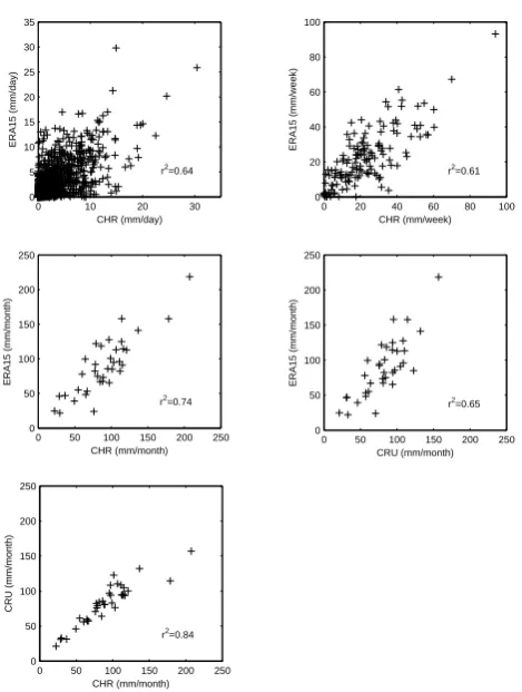
Rainfall amounts of the three forcing datasets were compared for the period of 1993–1995; the only three years the three datasets all overlap. A first comparison was made for basin wide mean values at a daily basis between the ERA15 and CHR values. For the second comparison, the ERA15 and CHR data sets were aggregated to weekly and monthly val-ues and then compared to the CRU data.
4.3 Model performance 4.3.1 Calibration at Lobith
As is explained in Sect. 4.1, HBV and VIC were forced both by ERA15 and CHR precipitation values for comparison rea-sons. For VIC this results in a forcing data set containing a combination of measured data for precipitation and RCM output for the remaining seven input parameters. This forc-ing dataset is considered incorrect and therefore both models were calibrated using only ERA15 output.
We forced both models with ERA15 data and calibrated for the discharge gauge at the Dutch-German border at Lo-bith (see Fig. 1c) using observed discharge at LoLo-bith for the year 1993. Only one year was used in order to limit the amount of calibration time for the VIC model. Because 1993 contains a relatively dry summer, as well as an extreme peak in winter, it was considered representative of the extremes for the total period. The model simulations were initialized using model states of October 1993 and also the first two months of 1993 are considered as a “warm-up” period, hence model results for this period were not used in the calibration process.
To calibrate VIC, former applications of VIC (Liang et al., 1994) were followed in that seven parameters were selected for calibration using an automated approach. These seven parameters describe the layer depths, relations between soil moisture content and baseflow and the infiltration capacity. For a complete description, see Hurkmans (2008).
The original calibration process for the HBV model of the Rhine basin is described by Eberle (2005). HBV was recal-ibrated for the year 1993 in a stepwise approach using the ERA15 dataset. Based on results of a parameter sensitivity analysis by Passchier and Stone (2003), for HBV, only the parameters fc (field capacity that represents the total water storage capacity of the soil) and khq (describing the quick runoff function) were adjusted for recalibration.
4.3.2 Sub-basin scale validation performance
Table 1. Basin and sub-basin characteristics. Surface area (km2)is defined by the basin area upstream of the gauging station.
Basin Gauge Surface area Mean Q Min. Q Max. Q Mean annual Data period
(km2) (m3s−1) (m3s−1) (m3s−1) max. Q(m3s−1)
Rhine Lobith 160 800 2 206 788 11 885 7473 1989–2005
Rhine Andernach 139 549 2116 618 10 406 6494 1961–2004
Mosel Cochem 27 088 334 10 4020 2190 1961–2004
Lahn Kalkofen 5304 48 0 730 364 1961–2004
Main Raunheim 27 142 176 44 1991 1043 1989–2005
Neckar Rockenau 12 710 141 3 2105 1133 1971–1990
Rhine Maxau 50 624 1297 379 4430 3191 1961–2004
0 10 20 30
0 5 10 15 20 25 30 35
CHR (mm/day)
ERA15 (mm/day)
0 20 40 60 80 100 0
20 40 60 80 100
CHR (mm/week)
ERA15 (mm/week)
0 50 100 150 200 250 0
50 100 150 200 250
CHR (mm/month)
ERA15 (mm/month)
0 50 100 150 200 250 0
50 100 150 200 250
CRU (mm/month)
ERA15 (mm/month)
0 50 100 150 200 250 0
50 100 150 200 250
CHR (mm/month)
CRU (mm/month)
r2=0.64 r2=0.61
r2=0.74
r2=0.65
r2=0.84
Fig. 2. ERA15 versus CHR versus CRU precipitation. The period 1993–1995 was used for the comparison.
choose from for model validation, such as those presented by Krause (2005) and each criterion may place different empha-sis on different types of simulated and observed behaviours. The objective performance criteria used in the current study to compare the integral time series for the locations, are the coefficient of efficiency (E)(Nash and Sutcliffe, 1970), the coefficient of determination (r2)and the volume error (V E). Model performance differs with the scale on which it is applied. In the present study we are interested in discharges
at Lobith (the outlet of the basin), discharges upstream in the main Rhine channel and model performance at the sub-basin scale. The discharge gauges that were used in the analysis are Lobith, Andernach and Maxau along the Rhine branch, and tributary gauging stations at Cochem (Moselle), Kalkofen (Lahn), Raunheim (Main) and Rockenau (Neckar). These locations are shown in Fig. 1 and characteristics of the sub-basins upstream of those gauges are presented in Table 1. 4.3.3 Peak flows and low flows
Periods with extreme discharges are often of most interest both in impact studies and real time flow predictions. A good representation by the model of the absolute amount, the timing and duration of the peak and low flows is very relevant. Subsequently, just for the gauge at Lobith, we se-lected five peak flow and five low flow periods, and chose additional performance indicators that relate to magnitude and timing of peak flows, together with minimum values and duration of low flows. These indicators are observed maxi-mum discharge (max.Qobs), relative difference between
ob-served and simulated maximum discharge (dmax.Qsim),
dif-ference in peak timing (dT), observed minimum discharge (min.Qobs), relative difference between observed and
simu-lated minimum discharge (dmax.Qsim)and duration of the
low flow period under a threshold of 1300 m3/s (DUT). A discharge of 1300 m3/s at Lobith is a critical value in summer periods; lower discharges affect shipping industry, agricul-tural supply, electricity production and drinking water sup-plies.
5 Results
5.1 Forcing data comparison
[image:6.595.51.286.232.543.2]Table 2. Performance criteria daily and monthly discharge values at Lobith for the calibration period (March 1993–December 1993) and the validation period (1994–2003).
Calibration period Validation period
daily monthly daily monthly
E VIC ERA15 0.47 0.26 0.31 0.40
HBV ERA15 0.49 −0.08 0.62 0.60
VIC CHR 0.44 0.35 – –
HBV CHR 0.85 0.73 – –
r2 VIC ERA15 0.64 0.58 0.54 0.67
HBV ERA15 0.75 0.54 0.65 0.64
VIC CHR 0.81 0.88 – –
HBV CHR 0.97 0.96 – –
VE VIC ERA15 0.23 0.23 0.08 0.08
HBV ERA15 0.32 0.32 −0.04 −0.04
VIC CHR −0.55 −0.55 – –
HBV CHR 0.19 0.19 – –
measured datasets are compared with ERA15 data. Figure 2 illustrates the correlation between the precipitation data at different time steps. Daily values of ERA15 and CHR cor-relate poorly (r2=0.41) while the correlation coefficient in-creases with increasing time step length. The precipitation values of the ERA15 data do not show a constant bias that can be corrected. The correlation between monthly values of ERA15 and CHR is reasonably well (r2=0.74) and slightly higher than between ERA15 and CRU (r2=0.65). The cor-relation between CHR and CRU, however, has anr2value of 0.84, which indicates that these two databases are most alike and that ERA15 probably has a larger error than the measured data.
5.2 Model performance
5.2.1 Calibration and validation period at Lobith
Daily values of all performance criteria for Lobith are dis-played in Table 2, where a distinction is made between the calibration and the validation period. The additional six lo-cations will be discussed in Sect. 5.2.2. At Lobith after cal-ibration, the results of the HBV model forced with ERA15 show a moderate performance (E=0.49, r2=0.75), whereas the VIC model fits less well (E=0.47, r2=0.64). This is mainly caused by an overestimation of the volume, by 23% (VIC) and 32% (HBV), respectively. VIC forced by CHR shows an increased correlation (r2=0.81) when compared to its performance when forced by ERA15, but a decrease on the other performance criteria (E=0.44, V E=–0.55). How-ever, the HBV model forced with CHR fits well when com-pared to observed discharges (E=0.85,r2=0.97).
Figure 4 depicts the results of the period 1993–2003 at Lobith, respectively for the VIC and the HBV models both forced with ERA15 data. The HBV model shows a
bet-0 100 200 300
P (mm)
P ERA15 P CHR
0 2000 4000 6000 8000 10000 12000
Q (m
3/s)
Mar Apr May Jun Jul Aug Sep Oct Nov Dec 0
2000 4000 6000 8000 10000 12000
1993
Q (m
3/s)
VIC ERA15 HBV ERA15 Observed
VIC CHR HBV CHR Observed
Fig. 3. Monthly precipitation values for the Rhine basin according to different datasets (top) and daily discharge values at Lobith (bot-tom); model simulation results for the calibration period compared to the observed discharge in the period March–December 1993.
−5000 0 5000
d
Q (m/s)
500 1000 1500 2000 2500 3000 3500 4000 0
2000 4000 6000 8000 10000 12000
Q (m/s)
−5000 0 5000
d
Q (m
3/s)
500 1000 1500 2000 2500 3000 3500 4000 0
2000 4000 6000 8000 10000 12000
T (days)
Q (m
3/s)
Observed Simulated VIC
[image:7.595.49.287.107.272.2]Observed Simulated HBV
Fig. 4. Daily simulation results of the HBV model (a) and the VIC model (b) compared to the observed river discharge for the period 1993–2003 (4017 days).
[image:7.595.311.544.340.572.2]Table 3. Observed and simulated mean, minimum and maximum discharge (in m3/s), their standard deviation (SD) and skewness for the period March 1993 through December 2003.
Basin Gauge MeanQ MinQ MaxQ SD Skewness
(m3/s) (m3/s) (m3/s) (m3/s) (–)
Rhine Lobith Observed 2387 788 11 885 1300 2.29
VIC 2811 773 11 394 1468 1.45
HBV 2339 746 11 228 1244 1.99
Rhine Andernach Observed 2197 630 10 500 1182 2.29
VIC 2474 734 10 487 1258 1.46
HBV 2054 593 11 092 1104 2.08
Mosel Cochem Observed 355 31 4020 416 3.20
VIC 325 49 2463 282 2.63
HBV 263 21 3644 274 4.37
Lahn Kalkofen Observed 48 0 598 61 3.86
VIC 42 6 350 42 2.44
HBV 33 1 506 40 4.21
Main Raunheim Observed 183 51 1,991 197 3.65
VIC 234 39 1885 227 2.48
HBV 180 44 1946 189 3.89
Neckar Rockenau Observed 150 27 2140 142 5.26
VIC 216 34 2490 201 3.17
HBV 144 19 2291 167 4.93
Rhine Maxau Observed 1322 400 4330 530 1.38
VIC 1631 374 5222 739 0.98
HBV 1335 407 5137 629 1.18
by VIC). A visual analysis of the hydrographs at multiple peak flow events, shows that both models simulate the re-cession curve well. Errors arise at most extreme peak events (see Sect. 5.2.3 on peak flows and low flows) where the quick flow component either is too small or too large. VIC tends to overestimate more peaks than HBV does and shows a de-layed peak at many peak events. Medium flows are mostly well represented by HBV, whereas VIC substantial over esti-mates discharges, sometimes for a period of several months. Low flow periods are simulated well for a length of time up to 2 or 3 months, and when drought periods are more lengthy, both models tend to underestimate baseflow (see Sect. 5.2.3). The changeable reaction of both models to different mete-orological conditions suggests that the storage capacity in the upper layers is very irregular, resulting in variable esti-mates of direct runoff. Also, the depletion factor controlling drainage from the lower layers seems to be too large dur-ing lengthy drought events. A further explanation for these moderately successful results might be that at a short time step like a daily basis, errors in timing of simulated high and low flows have a considerable negative influence on the performance indicators. Nonetheless, when monthly values of simulated discharge are evaluated they display similar or slightly worse results, as can be seen from Table 2; VIC and HBV forced with ERA15 perform moderate and HBV forced with CHR fits well, which is about equal to the HBV
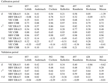
Table 4. Performance criteria daily discharge values.kmrrepresents the length of the Rhine from the Bodensee.
Calibration period
kmr 857 613 592 586 497 428 363
Lobith Andernach Cochem Kalkofen Raunheim Rockenau Maxau
E VIC ERA15 0.47 0.52 0.45 0.24 0.64 −0.16 −1.20 HBV ERA15 0.49 0.59 0.81 0.30 0.60 0.31 −0.40 VIC CHR 0.44 0.68 0.63 0.50 0.46 0.14 0.64 HBV CHR 0.85 0.91 0.92 0.86 0.89 0.77 0.78
r2 VIC ERA15 0.64 0.61 0.57 0.50 0.76 0.40 0.47 HBV ERA15 0.75 0.75 0.82 0.37 0.83 0.48 0.54 VIC CHR 0.81 0.81 0.69 0.67 0.78 0.52 0.71 HBV CHR 0.97 0.97 0.95 0.86 0.96 0.88 0.95
V E VIC ERA15 0.23 0.14 -0.31 -0.49 0.43 0.50 0.27 HBV ERA15 0.32 0.23 0.17 −0.31 0.62 0.28 0.22 VIC CHR −0.55 −0.07 −0.14 −0.52 −0.34 0.06 −0.41 HBV CHR 0.19 0.10 0.13 −0.08 0.21 0.12 0.09 Validation period
kmr 857 613 592 586 497 428 363
Lobith Andernach Cochem Kalkofen Raunheim Rockenau Maxau
E VIC ERA15 0.31 0.30 0.38 0.32 0.05 −0.46 −0.62 HBV ERA15 0.62 0.55 0.48 0.44 0.07 0.17 0.28
r2 VIC ERA15 0.54 0.48 0.43 0.43 0.27 0.32 0.39 HBV ERA15 0.65 0.60 0.56 0.51 0.23 0.45 0.49
V E VIC ERA15 0.08 0.02 −0.25 −0.36 0.02 0.21 0.18 HBV ERA15 −0.04 −0.09 −0.29 −0.31 −0.05 −0.07 −0.01
while observed and simulated discharge agree quite well. This lack of reaction in modelled discharge in August can be explained by higher evaporation values during summer than spring, which neutralize the precipitation surplus, next to the fact that absolute precipitation values are lower in summer than in springtime.
5.2.2 Sub-basin scale performance
Several statistical parameters for the complete simulation period are presented in Table 3. The mean and minimum simulated discharges agree reasonable well for the HBV model, whereas VIC overestimates those values, except for the gauges at Cochem and Kalkofen. The maximum dis-charges, though, are underestimated for most locations, ex-cept for the most upstream gauges Rockenau and Maxau. The values for the standard deviation (SD) based on daily values are high for both simulated and observed values. This can be explained by the skewed distribution of the discharge values. Based on this information it can be concluded that the probability density function of the observed values at Lobith is best represented by the simulated discharges by HBV.
For the remaining six gauges upstream of Lobith, scatter plots of the daily observed and simulated discharges are dis-played (Fig. 5) for the validation period. The accessoryr2
values are presented in Table 4. Tables 4 and 5 show the
results of all performance criteria for daily and monthly val-ues respectively, for all locations. Above the location name, the kmr number is displayed. This number represents the length of the Rhine from the Bodensee in Switzerland and Germany. For example, the gauging station at Lobith is lo-cated 857 km downstream form the Bodensee. In the current study, the gauges that are not located exactly along the Rhine, but along tributaries draining the sub-basins, have kmr num-bers that represent locations where the side rivers enter the Rhine. The kmr number is used to illustrate all performance criteria as presented in Tables 4 and 5, in a graphical way in Figs. 6 and 7. In Fig. 7, the volume error is not displayed, since the volume error does not change when the time step is adjusted (see Tables 4 and 5).
0 4000 8000 12000 0 2000 4000 6000 8000 10000 12000 Lobith
Q (m3/s) Observed
Q (m
3/s) VIC
0 4000 8000 12000 0 2000 4000 6000 8000 10000 12000 Lobith
Q (m3/s) Observed
Q (m
3/s) HBV
0 4000 8000 12000 0 2000 4000 6000 8000 10000 12000 12000 Andernach
Q (m3/s) Observed
Q (m
3/s) VIC
0 4000 8000 12000 0 2000 4000 6000 8000 10000 12000 Andernach
Q (m3/s) Observed
Q (m
3/s) HBV
0 1000 2000 3000 4000 0 1000 2000 3000 4000 Cochem
Q (m3/s) Observed
Q (m
3/s) VIC
0 1000 2000 3000 4000 0 1000 2000 3000 4000 Cochem
Q (m3/s) Observed
Q (m
3/s) VIC
0 200 400 600
0 200 400 600
Kalkofen
Q (m3/s) Observed
Q (m
3/s) VIC
0 200 400 600
0 200 400 600
Kalkofen
Q (m3/s) Observed
Q (m
3/s) HBV
0 500 1000 1500 2000 0 500 1000 1500 2000 Raunheim
Q (m3/s) Observed
Q (m
3/s) VIC
0 500 1000 1500 2000 0 500 1000 1500 2000 Raunheim
Q (m3/s) Observed
Q (m
3/s) HBV
0 500 1000 1500 2000 2500 0 500 1000 1500 2000 2500 Rockenau
Q (m3/s) Observed
Q (m
3/s) VIC
0 500 1000 1500 2000 2500 0 500 1000 1500 2000 2500 Rockenau
Q (m3/s) Observed
Q (m
3/s) HBV
0 2000 4000 6000
0 1000 2000 3000 4000 5000 6000 Maxau
Q (m3/s) Observed
Q (m
3/s) VIC
0 2000 4000 6000
0 1000 2000 3000 4000 5000 6000 Maxau
Q (m3/s) Observed
Q (m
[image:10.595.61.536.67.470.2]3/s) HBV
Fig. 5. Scatter plots of observed and simulated dischargeQ(m3/s) at a daily basis. The results for VIC are displayed on the left side and for
HBV on the right side.
basis, whereas VIC performs marginally better than HBV at a monthly basis. When studying the validation period on the right side, however, HBV performs substantially better than VIC, which indicates that HBV is more robust in its perfor-mance.
5.2.3 Peak flows and low flows
Table 6 shows the five highest daily discharges and the five lowest monthly discharges, as observed and simulated at Lo-bith. Observed volumes over threshold and maximum peak discharges reveal that both models overestimate and under-estimate the same peaks. Furthermore, it shows that VIC tends to delay flood peaks, for some peaks even up to 6 days, while HBV simulates the timing of the peaks very well. Two factors in VIC explain this delaying of peak flows: first, the routing algorithm that is used in VIC might delay
300 400 500 600 700 800 900 −1 −0.5 0 0.5 1
kmr
E (−)
300 400 500 600 700 800 900 0 0.2 0.4 0.6 0.8 1
kmr
r
2 (−)
300 400 500 600 700 800 900 −0.7 −0.5 −0.3 −0.1 0.1 0.3 0.5 0.7
kmr
VE (−)
300 400 500 600 700 800 900 −1.5
−1 −0.5 0 0.5 1
kmr
E (−) VIC ERA15 HBV ERA15 VIC CHR HBV CHR
300 400 500 600 700 800 900 0 0.2 0.4 0.6 0.8 1
kmr
r
2 (−)
300 400 500 600 700 800 900 −0.7 −0.5 −0.3 −0.1 0.1 0.3 0.5 0.7
kmr
[image:11.595.73.522.68.405.2]VE (−)
Fig. 6. Performance criteria daily discharge values. kmrrepresents the length of the Rhine from the Bodensee. The calibration period is
displayed at the left side and the validation period at the right side.
Concerning the low flows, VIC tends to underestimate the minimum values and HBV tends to overestimate the low flows under consideration. For the duration of the most ex-treme low flows below a threshold of 1300 m3/s, both mod-els underestimated the duration of the low flows significantly and showed variable performance on the less extreme low flow periods.
6 Discussion and conclusions
In the view of the utility of hydrological models in climate scenario studies, the goal of this paper was to compare the hydrological models HBV and VIC by testing their perfor-mance for simulating historical discharge in the Rhine basin. These models have different model structures and there is no consensus in research on rainfall-runoff modelling on what model structure is to be preferred. Some research suggest, however, that the VIC approach more accurately simulates the timing of peak discharges (Troy et al., 2007). Different meteorological data sets were used as model input and HBV
and VIC were compared at both basin and sub-basin scale using various performance criteria. Furthermore, simulated peak flows and low flows were compared.
We have seen that the performance of both models was less in upstream basins than at the basin outlet (gauging station Lobith), but that for all upstream basins HBV still performed better than VIC at a daily basis. We have seen that HBV was more robust when the performance of the calibration period (E=0.49, r2=0.75 vs.E=0.47, r2=0.64 at Lobith) and the validation period (E=0.62,r2=0.65 vs.E=0.31, r2=0.54 at Lobith) were compared. In addition, HBV forced with CHR data (E=0.85, r2=0.97 for the calibration period at Lobith) performed much better than VIC forced with CHR (E=0.44,
r2=0.81) and than both VIC and HBV forced with ERA15. For the most extreme peak flows, HBV simulated maxi-mum discharges best (dmax.QsimHBV 1–17%,dmax.Qsim
VIC 2–27%), while VIC performed better at the moderate peak flows (dmax. Qsim HBV 21–35%, dmax. Qsim VIC
300 400 500 600 700 800 900 −1.5
−1 −0.5 0 0.5 1
kmr
E (−)
300 400 500 600 700 800 900 0 0.2 0.4 0.6 0.8 1
kmr
r
2 (−)
300 400 500 600 700 800 900 −1.5
−1 −0.5 0 0.5 1
kmr
E (−)
300 400 500 600 700 800 900 0 0.2 0.4 0.6 0.8 1
kmr
r
2 (−)
[image:12.595.68.525.64.294.2]VIC ERA15 HBV ERA15 VIC CHR HBV CHR
Fig. 7. Performance criteria monthly discharge values.kmrrepresents the length of the Rhine from the Bodensee. The calibration period is
displayed at the left side and the validation period at the right side.
Table 5. Performance criteria monthly discharge values.kmrrepresents the length of the Rhine from the Bodensee.
Calibration period
kmr 857 613 592 586 497 428 363
Lobith Andernach Cochem Kalkofen Raunheim Rockenau Maxau
E VIC ERA15 0.26 0.41 0.54 0.21 0.58 0.05 −1.39 HBV ERA15 −0.08 0.22 0.78 0.13 0.32 −0.09 −0.71 VIC CHR 0.35 0.61 0.55 0.50 0.68 0.31 0.59 HBV CHR 0.73 0.88 0.96 0.97 0.91 0.79 0.72
r2 VIC ERA15 0.58 0.57 0.86 0.61 0.82 0.70 0.50 HBV ERA15 0.54 0.58 0.83 0.20 0.77 0.30 0.48 VIC CHR 0.88 0.65 0.65 0.95 0.89 0.85 0.92 HBV CHR 0.96 0.97 0.98 0.97 0.98 0.93 0.96
V E VIC ERA15 0.23 0.14 −0.31 −0.49 0.43 0.50 0.27 HBV ERA15 0.32 0.23 0.17 −0.31 0.62 0.28 0.22 VIC CHR −0.55 −0.07 −0.14 −0.52 −0.34 0.06 −0.41 HBV CHR 0.19 0.10 0.13 −0.08 0.21 0.12 0.09 Validation period
kmr 857 613 592 586 497 428 363
Lobith Andernach Cochem Kalkofen Raunheim Rockenau Maxau
E VIC ERA15 0.40 0.42 0.55 0.34 0.40 −0.86 −0.62 HBV ERA15 0.60 0.52 0.48 0.41 0.48 0.32 0.28
r2 VIC ERA15 0.67 0.62 0.64 0.53 0.67 0.64 0.39 HBV ERA15 0.64 0.60 0.62 0.54 0.59 0.60 0.49
[image:12.595.113.486.388.673.2]Table 6. Analysis of peak flows and low flows at the outlet of the basin (Lobith), showing observed maximum discharge (max.Qobs),
relative difference between observed and simulated maximum discharge (dmax.Qsim), difference in peak timing (dT), observed minimum
discharge (min.Qobs), relative difference between observed and simulated minimum discharge (dmax.Qsim)and duration of the low flow
period under a threshold of 1300 m3/s (DUT).
Peak flows 31/01/1995 25/12/1993 04/11/1998 07/01/2003 28/03/2001
Max.Qobs(m3/s) 11 775 11 034 8410 9366 8666
dmax.QsimVIC (%) −26.7 1.5 −35.1 −15.5 −12.5
dmax.QsimHBV (%) −16.3 0.9 −34.9 −32.1 −20.6
dT VIC (days) 2 2 6 5 4
dT HBV (days) 0 0 0 −1 −1
Low flows 09/2003 11/1997 08/1998 09/1996 03/1993
Min.Qobs(m3/s) 788 931 983 1077 1228
dmin.QsimVIC (%) −20.3 −10.7 4.5 −26.0 −38.5
dmin.QsimHBV (%) 18.7 6.5 44.4 −15.8 0.5
DUTQobs(days) 141 68 39 37 13
DUT VIC (days) 104 22 15 60 68
DUT HBV (days) 93 33 0 54 11
discharge. Most low flows were underestimated by VIC, where HBV showed overestimation of the low flows. Also the performance of both models in reproducing duration of low flows was poor.
Hence, the semi-distributed lumped conceptual HBV model performed much better than the distributed land sur-face model VIC. This deflects from the general idea that more complex distributed modelling better represents ob-served discharges as compared to simple conceptual model approaches (Reggiani and Schellekens, 2003; Refsgaard, 1996). These results support the notion that even for a well documented river basin such as the Rhine, more com-plex modelling does not automatically lead to better results (Booij, 2003; Uhlenbrook, 2003).
We are convinced, though, that VIC should be able to per-form better than it has done so far in the Rhine basin, and thus model performance might be improved (Hurkmans et al., 2008). The performance of VIC might increase using a longer calibration period and further refining the spatial dis-tribution of adjusted parameters. Furthermore, by solving both the water and the energy balance VIC holds the poten-tial to better describe soil-atmosphere feedback processes, if the model scheme were to be combined with an atmo-spheric model. In the line of small-scale hydrometeorology and modelling the effects of land use change, this is a conclu-sive reason for further development (Hurkmans et al., 2008). Moreover, VIC has performed well in the past, for example in studies by Liang et al. (1994) and Troy et al. (2007). But also the HBV model for the Rhine basin can be improved. Lake retention for example, is not implemented yet in both models. Especially concerning the Bodensee, a large upstream lake in the Rhine basin, this is a quite drastic simplification and an obvious potential for further improvement. We subscribe the
recommendation of Seibert (1999), that model development and calibration is an undertaking that should not be carried out by a single researcher, but requires scientific dialogue.
The results also lead us to the conclusion that forcing data has a considerable influence on model performance, irrespec-tively to the type of model structure. It emphasizes the need for ground-based meteorological measurements and a sug-gestion might be to correct downscaled climate model re-analysis data such as ERA15, whenever measurements are available. It should be kept in mind that comparing mean val-ues of precipitation and temperature provides little guide to the quality of the data during more extreme events that affect hydrological systems. Pitman and Perkins (2007), for exam-ple, propose a probability density function based assessment and a skill score that shows a climate model’s ability to simu-late the 95th rainfall percentile. Comprehensive comparison and correction of downscaled climate model output is a chal-lenging task for further research.
Acknowledgements. This research was supported by the project ACER (A7) under the Dutch BSIK Climate Changes Spatial
Planning program. We wish to thank H. Buiteveld from the
Dutch Institute for Inland Water Management and Waste Water Treatment (RIZA) and the German Federal Institute of Hydrology (BfG) for both allowing the use of the HBV model, and providing
meteorological and discharge measurement data. D. Jacob and
E. Mazurkewitz from the Max Planck Institute for Meteorology are kindly acknowledged for providing meteorological data. Finally we thank two anonymous colleagues for occasional data editing and their constructive comments that helped to improve this paper.
Edited by: E. Todini
References
Abbott, M. B., Bathurs, J. C., Cunge, J. A., O’Connel, P. E., and Rasmussen, J.: An introduction to the european hydrological sys-tem – syssys-teme hydrologique “She”, 1: History and philosophy of a physically based distributed modelling system, J. Hydrol., 87, 45–59, 1986.
Bergstr¨om, S.: Development and application of a conceptual runoff model for scandinavian catchments, ph.D. Thesis, Department of water resources engineering, University of Lund, Lund, Sweden, 1976.
Bergstr¨om, S., Lindstr¨om, G., and Pettersson, A.: Multi-variable parameter estimation to increase confidence in hydrological modelling, Hydrol. Process., 16, 413–421, 2002.
Beven, K.: How far can we go in distributed hydrological mod-elling?, Hydrol. Earth Syst. Sci., 5, 1–12, 2001,
http://www.hydrol-earth-syst-sci.net/5/1/2001/.
Beven, K.: Towards an alternative blueprint for a physically based digitally simulated hydrologic response modelling system, Hy-drol. Process., 16, 189–206, 2002a.
Beven, K.: Towards a coherent philosophy for modelling the envi-ronment, Proc. R. Soc. Lond. A, 458, 1–20, 2002b.
Bogaard, T. A., Luxemburg, W. M. J., De Wit, M., Douben, N., and Savenije, H. H. G.: Some hydrological challenges in under-standing discharge generation processes in the Rhine and Meuse basins, Phys. Chem. Earth, 30, 262–266, 2005.
Booij, M. J.: Determination and integration of appropriate spatial scales for river basin modelling, Hydrol. Process., 17, 2581– 2598, 2003.
Buishand, T. A. and Lenderink, G.: Estimation of future discharges of the river Rhine in the SWURVE project, KNMI, De Bilt, The Netherlands TR-273, 1–36, 2004.
De Roo, A. P. J., Wesseling, C. G. and Van Deursen, W. P. A. Physically based river basin modelling within a GIS. The LIS-FLOOD model. Proc. 3rd Int. Conf. on Geo-Computation. In: Geo-Computation CF-ROM produced by R. J. Abrahart, 1998. De Roo, A. P. J., Wesseling, C. G. and Van Deursen, W. P. A.
Phys-ically based river basin modelling within a GIS. The LISFLOOD model. Hydrol. Process., 14, 1981–1992, 2000.
Disse, M. and Engel, H.: Flood events in the Rhine basin: Genesis, influendes and mitigation, Nat. Hazards, 23, 271–290, 2001. The water page – the Rhine river: http://www.thewaterpage.com/
rhine main.htm, access: 2 April 2007, 2001.
Eberle, M., Buiteveld, H., Wilke, K., and Krahe, P.: Hydrolog-ical modelling in the river Rhine basin part III - daily HBV model for the Rhine basin, Institute for Inland Water Manage-ment and Wase Water TreatManage-ment (RIZA) and Bundesanstalt f¨ur Gew¨asserkunde (BfG), Koblenz, Germany BfG-1451, 2005. Hurkmans, R. T. W., De Moel, H., Aerts, J. C. J. H., and Troch,
P. A.: Water balance versus land surface model in the simula-tion of Rhine river discharges, Water Resour. Res., 44, W01418, doi:10.1029/2007WR006168, 2008.
Jacob, D.: A note to the simulation of the annual and inter-annual variability of the water budget over the baltic sea drainage basin, Meteorol. Athos. Phys., 77, 61–73, 2001.
Jothityangkoon, M., Sivalapan, M., and Farmer, D. L.: Process con-trols of water balance variability in a large semi-arid catchment: Downward approach to hydrological model development, J. Hy-drol., 254, 174–198, 2001.
Krause, P., Boyle, D. P. and B¨ase, F.: Comparison of different effi-ciency criteria for hydrological model assessment, Adv. Geosci., 5, 89–97, 2005,
http://www.adv-geosci.net/5/89/2005/.
Kundzewicz, Z. W., Mata, L. J., Arnell, N. W., D¨oll, P., Kabat, P., Jim´enez, B., Miller, K. A., Oke, T., Sen, Z., and Shiklomanov, I. A.: Freshwater resources and their management, in: Climate change 2007: Impacts, adaptation and vulnerability, Contribu-tion of working group ii tot the fourth assessment report of the intergovernmental panel on climate change, edited by: Parry, M. L., Conziani, O. F., Palutikof, J. P., Van der Linden, P. J., and Hanson, C. E., Cambridge University Press, Cambridge, UK, 173–210, 2007.
Kwadijk, J. C. J.: The impact of climate change on the discharge of the river Rhine, PhD Thesis, University of Utrecht, Utrecht, The Netherlands, 1993.
Liang, X., Lettenmaier, D. P., Wood, E. F., and Burges, S. J.: A simple hydrologically based model of land surface water and en-ergy fluxes for general circulation models, J. Geophys. Res., 99, 415–428, 1994.
Liang, X., and Zhenghui, X.: A new surface runoff parameteriza-tion with subgrid-scale soil heterogeneity for land surface mod-els, Adv Water Resour, 24, 1173-1193, 2001.
Lindstr¨om, G., Johansson, B., Persson, M., Gardelin, M., and Bergstr¨om, S.: Development and test of the distributed HBV-96 hydrological model, J. Hydrol., 201, 272–288, 1997.
Liu, Z. and Todini, E. Towards a comprehensive physically-bassed rainfall-runoff model. Hydrol. Earth Syst. Sci., 6, 859–881, 2002, http://www.hydrol-earth-syst-sci.net/6/859/2002/.
Lohmann, D., Nolte-Holube, R., and Raschke, E.: A
large-scale horizontal routing model to be coupled to land surface parametrization schemes, Tellus, 48A, 708–721, 1996.
Middelkoop, H., Daamen, K., Gellens, D., Grabs, W., Kwadijk, J. C. J., Lang, H., Parmet, B. W. A. H., Sch¨adler, B., Schulla, J., and Wilke, K.: Impact of climate change on hydrological regimes and water resources management in the Rhine basin., Climatic Change, 49, 105–128, 2001.
Mitchell, T. D. and Jones, P. D.: An improved method of construct-ing a database of monthly climate observations and associated high-resolution grids, Int. J. Climatol., 25, 693–712, 2005. M¨ulders, R., Parmet, B., and Wilke, K.: Hydrological modelling in
Nash, J. E. and Sutcliffe, J. V.: River flow forecasting through con-ceptual models. Part i – a discussion of principles, J. Hydrol., 10, 282–290, 1970.
Passchier, R. and Stone, K.: Analysis of the instrumentation for
computing design discharges, WL|Delft Hydraulics, Delft, The
Netherlands, Q2705, 1–78, 2003.
Perrin, C., Michel, C., and Andr´eassian, V.: Does a large num-ber of parameters enhance model performance? Comparative as-sessments of common catchment model structures on 429 catch-ments, J. Hydrol., 242, 275–301, 2000.
Pitman, A. J. and Perkins, S. E.: Reducing uncertainty in se-lecting climate models for hydrological impact assessments, in: Quantification and Reduction of Predictive Uncertainty for Sus-tainable Water Resource Management, Symposium HS2004 at IUGG2007, Perugia, 3–15, 2007.
Refsgaard, J. C.: Terminology, modelling protocol and classifica-tion of hydrological model codes, in: Distributed hydrological modelling, edited by: Abbott, M. B. and Refsgaard, J. C., Kluwer Academic Publishers, 17–39, 1996.
Reggiani, P., Hassanizadeh, S. M., Sivapalan, M., and Gray, W. G.: A unifying framework for watershed thermodynamics: Balance equations for mass, momentum, energy and entropy, and the sec-ond law of thermodynamics, Adv. Water Resour., 22, 367–398, 1998.
Reggiani, P., Hassanizadeh, S. M., Sivapalan, M., and Gray, W. G.: A unifying framework for watershed thermodynamics: Constitu-tive relationships, Adv. Water Resour., 23, 15–39, 1999. Reggiani, P. and Schellekens, J.: Modelling of hydrological
re-sponses: The respresentative elementary watershed approach as an alternative blueprint for watershed modelling, Hydrol. Pro-cess., 17, 3785–3789, 2003.
Rientjes, T. and Zaadnoordijk, W. J.: Hoogwatervoorspelling: Fy-sisch gebaseerde regen-afvoermodellering. Dilemma of d´ej`a vu?, Stromingen, 6, 33–44, 2000 (in Dutch).
Savenije, H. G.: Equifinality, a blessing in disguise?, Hydrol. Pro-cess., 15, 2835–2838, 2001.
Sch¨ar, C., L¨uthi, D., Beyerly, U., and Heise, E.: The
soil-precipitation feedback: A process study with a regional climate model, J. Climate, 12, 722–741, 1998.
Schulla, J. and Kaspar, K.: Model description WaSIM-ETH, Inter-nal report, IAC, ETH, Z¨urich, 1–174, 2006.
Seibert, J.: Conceptual runoff models - fiction or representation of reality, MSc Thesis, Acta University, Uppsala, Sweden, 52 pp., 1999.
Shaw, E. M.: Hydrology in practice, Nelson Thornes Ltd, Chel-tenham, England, 1–569, 2002.
Sprokkereef, E.: Eine hydrologische datenbank f¨ur das Rheinge-biet, International Commission for the Hydrology of the Rhine Basin (CHR), 2001.
Te Linde, A. H.: Effect of climate change on the discharge of the rivers Rhine and Meuse. Applying the KNMI 2006 scenarios
us-ing the HBV model, WL|Delft Hydraulics, Delft, The
Nether-lands Q4286, 1–30, 2007.
Troy, T., Sheffield, J., and Wood, E.: Temporal and spatial scales in hydrological model calibration, in: Geophysical Research Ab-stracts, European Geosciences Union General Assembly 2007, Vienna, Austria, 2007,
Uhlenbrook, S., Seibert, J., Leibundgut, C., and Rodhe, A.: Pre-diction uncertainty of conceptual rainfall-runoff models caused by problems to identify model parameters and structure, Hydrol. Sci., 44, 779–798, 1999.
Uhlenbrook, S.: An emperical approach for delineating spatial units with the same dominating runoff generation processes, Phys. Chem. Earth, 28, 297–303, 2003.
Van Deursen, W. P. A. and Kwadijk, J. C. J.: Rhineflow: An inte-grated GIS water balance model for the river Rhine, HydroGIS 93: Application of Geographic Information Systems in Hydrol-ogy and Water Resources, 507–518, 1993.
Van Deursen, W. P. A.: Rapportage Rhineflow/Meuseflow. Nieuwe KNMI scenario’s mei 2006,, Carthago Consultancy, Rotterdam, the Netherlands, 2006 (in Dutch).
Vivoni, E. R. Hydrologic modeling using triangulated irregular net-works: terrain representation, flood forecasing and catchment response, PhD Thesis, Cambridge – Massaschusetts Institute of Technology, USA, 2003.
Wagener, T., McIntyre, N., Lees, M. J., Wheater, H. S., and Gupta, H. V.: Towards reduced uncertainty in conceptual rainfall-runoff modelling: Dynamic identifiability analysis, Hydrol. Process., 17, 455–476, 2003.
Ward, R. C. and Robinson, M.: Principles of hydrology, 4 ed., McGraw-Hill Publishing Company, London, 2000.
Weerts, A. H.: Assessing and quantifying the combined effect of model parameter and boundary uncertainties in model based flood forecasting., Geophys. Res. Abstr., 5, 14564, 2003. Weerts, A. H. and Van der Klis, H.: FEWS-Rhine version 1.02.
Improvements and adjustments., WL|Delft Hydraulics, Delft,
Q3618, 2004.