www.hydrol-earth-syst-sci.net/19/4113/2015/ doi:10.5194/hess-19-4113-2015
© Author(s) 2015. CC Attribution 3.0 License.
Rainfall erosivity estimation based on rainfall data collected
over a range of temporal resolutions
S. Yin1,2, Y. Xie1,2, B. Liu1,2, and M. A. Nearing3
1State Key Laboratory of Earth Surface Processes and Resource Ecology, Beijing Normal University, Beijing 100875, China 2School of Geography, Beijing Normal University, Beijing 100875, China
3USDA-ARS Southwest Watershed Research Center, Tucson, AZ 85719, USA Correspondence to: S. Yin ([email protected])
Received: 22 April 2015 – Published in Hydrol. Earth Syst. Sci. Discuss.: 20 May 2015 Revised: 11 September 2015 – Accepted: 27 September 2015 – Published: 9 October 2015
Abstract. Rainfall erosivity is the power of rainfall to cause soil erosion by water. The rainfall erosivity index for a rain-fall event (energy-intensity values –EI30) is calculated from
the total kinetic energy and maximum 30 min intensity of in-dividual events. However, these data are often unavailable in many areas of the world. The purpose of this study was to develop models based on commonly available rainfall data resolutions, such as daily or monthly totals, to calculate rain-fall erosivity. Eleven stations with 1 min temporal resolution rainfall data collected from 1961 through 2000 in the eastern half of China were used to develop and calibrate 21 mod-els. Seven independent stations, also with 1 min data, were utilized to validate those models, together with 20 previously published equations. The models in this study performed bet-ter or similar to models from previous research to estimate rainfall erosivity for these data. Using symmetric mean ab-solute percentage errors and Nash–Sutcliffe model efficiency coefficients, we can recommend 17 of the new models that had model efficiencies≥0.59. The best prediction capabili-ties resulted from using the finest resolution rainfall data as inputs at a given erosivity timescale and by summing results from equations for finer erosivity timescales where possible. Results from this study provide a number of options for de-veloping erosivity maps using coarse resolution rainfall data.
1 Introduction
Soil erosion prediction models are effective tools for helping to guide and inform soil conservation planning and practice. The most widely used soil erosion models used for
conserva-tion planning are derived from the Universal Soil Loss Equa-tion (USLE) (Wischmeier and Smith, 1965, 1978). These models include the USLE, the Revised USLE (RUSLE) (Re-nard et al., 1997), and RUSLE2 (Foster, 2004). Adaptations of the USLE have also been developed for use in other parts of the world, including, for example, Germany (Schwert-mann et al., 1990), Russia (Larionov, 1993), and China (Liu et al., 2002). For example, the Chinese Soil Loss Equation (CSLE) was used in the first national water erosion sample survey in China (Liu et al., 2013).
These models have in common a rainfall erosivity factor (R), which reflects the potential capability of rainfall to cause soil loss from hillslopes, and which is one of the most impor-tant basic factors for estimating soil erosion. In its simplest form, theRfactor is an average annual value, calculated as a summation of event-based energy-intensity values (EI30) for
a location divided by the number of years over which the data were collected.EI30is defined as the product of kinetic
en-ergy of rainfall and the maximum contiguous 30 min rainfall intensity during the rainfall event. It is the basic rainfall ero-sivity index that was developed by Wischmeier (1958) origi-nally for the USLE, and is still widely used in other erosion prediction models (e.g., RUSLE, RUSLE2), with some mod-ifications and improvements. Wischmeier (1976) suggested that more than 20 years’ rainfall data are needed to calculate average annual erosivity to include relatively dry and wet pe-riods.
rainfall record (e.g., 5 min) for a storm. Determination of the kinetic energy of a storm is more complex.
Kinetic energy (KE) is generally suggested to indicate the ability of a raindrop to detach soil particles from a soil mass (e.g., Nearing and Bradford, 1985). Since the direct measure-ment of KE requires sophisticated and costly instrumeasure-ments, several different estimating methods have been developed that estimate KE based on rainfall intensity (I) using loga-rithmic, exponential, or power functions. The original 1978 release of the USLE utilized a logarithmic function (Wis-chmeier and Smith, 1978) that was based on rainfall energy data published by Laws and Parsons (1943). Brown and Fos-ter (1987) re-evaluated this relationship and recommended the use of an exponential relationship, which was subse-quently used in RUSLE (Renard et al., 1997). For RUSLE2 Foster (2004) used the exponent value of−0.082, rather than the−0.05 value used in RUSLE, as follows:
er =0.29[1−0.72 exp(−0.082ir)], (1) where er is the estimated unit rainfall kinetic energy (MJ ha−1mm−1) andir is the rainfall intensity (mm h−1) at any given time within a rainfall event (usually taken as 1 min for computational purposes, with average-intensity represen-tative of the time increment). This was based largely on work of McGregor and Mutchler (1976) and McGregor et al. (1995), who found that the RUSLE equation gave values that were too low. The energy term used in RUSLE2 gives results on the order of those from the original USLE method. The temporal resolution of rainfall data available across the world does not always allow for a direct computation of rainfall kinetic energy (Sadeghi et al., 2011; Sadeghi and Tavangar, 2015; Oliveira et al., 2012; Panagos et al., 2015; Zhang and Fu, 2003), even within countries with extensive rainfall monitoring programs. In the United States, for exam-ple, intra-storm, temporally detailed data (historically taken on pen recording charts, now taken as 1 min digital data) are only available at limited stations, whereas daily data are common (Nicks and Lane, 1995; Flanagan et al., 2001). Yet there is a need for developing models for application in all areas of the world in order to produce erosivity maps that can be used for evaluating soil erosion rates (e.g., Sadeghi et al., 2011, Sadeghi and Tavangar, 2015; Oliveira et al., 2012; Panagos et al., 2015; Zhang and Fu, 2003). For that reason many efforts have been undertaken to estimate rain-fall erosivity by using daily (Richardson et al., 1983; Yu, 1998; Capolongo et al., 2008; Yin et al., 2007; Zhang et al., 2002a, b; Xie et al., 2001, 2015), monthly (Arnoldus, 1977; Renard and Freimund, 1994; Yu and Rosewell, 1996; Ferro et al., 1999; Wu, 1994; Zhou et al., 1995), or annual rain-fall data (Lo et al., 1985; Renard and Freimund, 1994; Yu and Rosewell, 1996; Bonilla and Vidal, 2011; Zhang and Fu, 2003; Wang, 1987; Sun, 1990). Generally the technique has been to develop a simple empirical relationship between ero-sivity and coarse resolution rainfall based on limited finer resolution data and then to extend the analyses to wider areas
and longer periods with coarser temporal resolution rainfall data (Angulo-Martinez and Begueria, 2012; Ma et al., 2014; Ramos and Duran, 2014; Sanchez-Moreno et al., 2014).
Several studies evaluated different timescales of erosivity using different temporal resolutions of rainfall data. In Eu-rope, Panagos et al. (2015) undertook the task to develop an erosivity map for Europe based on data from 1541 precipita-tion staprecipita-tions with temporal resoluprecipita-tions of 5 to 60 min. To use data that had been reported at the different time resolutions they had to apply adjustment factors to the data, which they reported to have introduced some uncertainty into the estima-tions. Sadeghi and Tavangar (2015) evaluated various erosiv-ity estimation indices, including Fournier (Fournier, 1960), modified Fournier (Arnoldus, 1977), Roose (1977) and Lo et al. (1985), using data from 14 stations in Iran. They eval-uated annual, seasonal, and monthly information. Similarly, the work in Brazil summarized by Oliveira et al. (2012) high-lighted several studies that used various estimations of ero-sivity based on various types of data and interpolations. Other innovative ways have been advanced to produce better map-pings of erosivity, including the use of daily (Fan et al., 2013) or 3 h (Vrieling et al., 2010, 2014) data from the Tropical Rainfall Measuring Mission (TRMM) Multi-satellite Precip-itation Analysis (TMPA) precipPrecip-itation data.
In China the specifications for surface meteorological observations by the China Meteorological Administration (China Meteorological Administration, 2003) have required since the 1950s that the maximum 60 and 10 min rainfall amounts, (P60)day and (P10)day, be compiled; hence, these
data are readily available in China. The measurements were made using siphon-method, self-recording rain gauges. Be-cause of this, there is an interest in China to utilize the max-imum daily 10 and 60 min rainfall intensities, (I10)day and
(I60)day, to calculate erosivity.
2 Data and methods 2.1 Data
Data collected at 18 stations by the Meteorological Bu-reaus of Heilongjiang, Shanxi, Shaanxi, Sichuan, Hubei, Fu-jian, and Yunnan provinces and the municipality of Beijing were used (Fig. 1, Table 1). These stations were distributed over the eastern half of China; 1 min resolution rainfall data (Data M) were obtained by using a siphon, self-recording rain gauge. The data collection period began in 1971 for Wuzhai (53663) and Yangcheng (53975) in Shanxi Province and from 1961 for the remaining 16 stations; the data records ended in 2000 for all stations. Quality control of Data M was done to select the best observation years using the more com-plete data sets of daily rainfall totals, Data D, which were observed by simple rain gauges at the same stations. Data M was compared with Data D on a day-by-day basis, and those days with deviation exceeding a certain criterion were marked as questionable and were not used in this analysis (Wang et al., 2004). The criterion used was that the data were considered good when the absolute deviation between Data M and Data D was less than 0.5 mm when the daily rainfall amount was less than 5 mm and no more than 10 % when the daily rainfall amount was greater than or equal to 5 mm. Data M in the earlier years of record tended to have more days with missing or suspicious observations. These totals of Data M and Data D were compared year-by-year to deter-mine which years could be designated as common years for use in this study, with an effective year having a relative devi-ation for yearly rainfall amount of no more than 15 %. There were at least 29 common years for all 18 stations, and seven stations had common years of at least 38 years (Table 1). Note that though there were missing data in the information used, Data D was only used for quality control purposes and the data used in the analysis, Data M, were internally consis-tent in that only the data from common years were used in all comparisons and evaluations reported.
Data M was used to calculate the event-basedEI30values
as a function of the calculated kinetic energy and maximum 30 min rainfall intensity (Foster, 2004). These were treated as observed values and summed to obtain the erosivity factors, R, for daily, month (individual month totals), year (individ-ual year totals), average monthly (one value for each month at each station), and average annual (one value for each sta-tion) timescales. Total rainfall event depth values were also compiled into the other temporal resolutions of rainfall data, including correspondent daily, month, year, average monthly, and average annual resolutions. For the eight stations in the northern part of China (including stations in Heilongjiang, Shanxi, Shaanxi provinces and Beijing municipality), only the periods from May through September were used because the siphon, self-recording rain gauges were not utilized in the winter to avoid freeze damage. Percentages of precipitation during May through September to total annual precipitation
varied from 75.6 to 89.2 % for these eight northern stations. Data M for the full 12 month year was used from the remain-ing 10 stations located in the southern parts of China.
Eleven stations, including Nenjiang, Wuzhai, Suide, Yan’an, Guangxiangtai, Chengdu, Suining, Neijiang, Fangx-ian, Kunming, and Fuzhou, marked with dots in Fig. 1, were used to calibrate the models (Table 1). The other seven stations, including Tonghe, Yangcheng, Miyun, Xichang, Huangshi, Tengchong, and Changting, marked with triangles in Fig. 1, were used to validate the models.
2.2 Calculation of the R factor at different timescales Different timescales for RUSLE2 erosivity, R, including event, daily, month, year, average monthly, and average an-nual, were calculated based on the 1 min resolution data (Data M). Recall that month and year refer to individual months and years, and not averages.EI30(MJ mm ha−1h−1)
is the rainfall erosivity index for a rainfall event, whereEis the total rainfall kinetic energy during an event andI30 is
the maximum contiguous 30 min intensity during an event (Wischmeier and Smith, 1978). An individual rainfall event was defined as a period of rainfall with at least six preceding and six succeeding non-precipitation hours (Wischmeier and Smith, 1978). An erosive rainfall event was defined as one with rainfall amounts greater than or equal to 12 mm, follow-ing Xie et al. (2002). We used the equation recommended by Foster 2004) for RUSLE2 to calculate the kinetic energy of the storms, which used Eq. (1) combined with
E= n X
r=1
(er·Pr) , (2)
whereer is the estimated unit rainfall kinetic energy (from Eq. 1) for therth minute (MJ ha−1mm−1);Pr is the 1 min rainfall amount for therth minute (mm);r=1, 2,. . .,n rep-resents each 1 min interval in the storm; andir is the rain-fall intensity for therth minute (mm h−1). The Foster (2004) equations were chosen because they are currently used for erosion assessment for RUSLE2 in the United States and for the CSLE in China, and it appears to give results similar to the original USLE, as was discussed in the Introduction.
Our evaluation included four models for events and one for daily erosivities. Event models were simply models to pre-dict individual event erosivities, regardless of whether they occurred in 1 or more days, and regardless of whether more than one event occurred in a day. For the daily model, rain-fall erosivity for each day,Rday, was calculated following the
method by Xie et al. (2015). When a day had only one ero-sive event and this event began and finished during the same day, then
Figure 1. Locations of the 18 stations with 1 min resolution rainfall data. Eleven stations marked with dots were used to calibrate 21 models. The other seven stations marked with triangles were used to validate models and conduct comparisons with previous research.
When more than one full rainfall event happened during 1 day, then
Rday= n X
i=1
Eevent_i·(I30)event_i, (4)
wherenis the number of rainfall events during the day, and Eevent_i and (I30)event_i are the total rainfall energy and the maximum contiguous 30 min intensity, respectively, for the ith event. When only one part of a rainfall event occurred during 1 day, then
Rday=Eday_d·(I30, )event, (5)
whereEday_d is the rainfall energy generated by the part of rainfall occurred during thedth day and (I30)eventis the
max-imum contiguous 30 min intensity for the entire event. The remaining situations were calculated by combining Eqs. (4) and (5).
Month, year, average monthly, and average annualR val-ues were summed from the event EI30 index by erosive
storms that occurred during the corresponding period. They
were calculated by using Eqs. (6)–(9).
Rmonth, y, m= J X
j=0
(EI30)y, m, j, (6)
Rave_month, m= 1 Y
Y X
y=1
Rmonth, y, m, (7)
Ryear, y= 12 X
m=1
Rmonth, y, m, (8)
Rave_annual= Y X
y=1
Ryear, y, (9)
whereyis the number of years of record; (EI30)y, m, j is the EI30 value for the jth event in themth month of the yth
year; Rmonth, y, m is the R value for the mth month of the yth year; Rave_month, m is the averageR value for the mth
month over the years of record; Ryear, y is R value in the yth year; andRave_annualrepresents average annual erosivity,
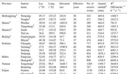
Table 1. Information for the 18 rainfall stations.
Province Station Lat. Long. Elevation Effective No. of Annual R4
name (◦N) (◦E) (m) years erosive rainfall3 (MJ mm ha−1 events (mm) h−1a−1)
Heilongjiang1 Nenjiang 49.17 125.23 243.0 30 343 485.8 1368.7 Tonghe2 45.97 128.73 110.0 38 471 596.2 1632.5 Shanxi1 Wuzhai 38.92 111.82 1402.0 30 289 464.0 781.9
Yangcheng2 35.48 112.4 658.8 30 340 605.9 1503.3 Shaanxi1 Suide 37.5 110.22 928.5 29 256 449.7 992.8
Yan’an 36.6 109.5 958.8 39 411 534.6 1233.7 Beijing1 Guanxiangtai 39.93 116.28 54.7 40 434 575.0 3188.1 Miyun2 40.38 116.87 73.1 37 476 648.1 3575.0 Sichuan Chengdu 30.67 104.02 506.1 39 717 891.8 3977.0 Xichang2 27.9 102.27 1590.9 40 998 1007.5 3021.0 Suining 30.5 105.58 279.5 33 654 932.7 4091.3 Neijiang 29.58 105.05 352.4 39 826 1034.1 5097.9 Hubei Fangxian 32.03 110.77 427.1 31 563 829.5 2298.4 Huangshi2 30.25 115.05 20.6 32 898 1438.5 6049.4 Yunnan Tengchong2 25.02 98.5 1648.7 36 1205 1495.7 3648.9 Kunming 25.02 102.68 1896.8 33 747 1018.8 3479.0 Fujian Fuzhou 26.08 119.28 84.0 39 1136 1365.4 5871.1 Changting2 25.85 116.37 311.2 31 1037 1728.1 8258.5
1The eight stations in these provinces are located in the northern part of China and had 1 min resolution data collected from May through September. The
remaining ten stations were based on data collected during the entire year.2Seven validation stations (the other 11 stations were calibration stations.)3
Based on daily rainfall data sets collected during 1961–2000.4Rin this case is the average annual erosivity.
2.3 Model calibration using different resolutions of rainfall data
A total of 21 models were calibrated for different timescales ofR, based on varying resolutions of rainfall data (Table 2). Event amountPeventand peak-intensity indices were derived
based on the 1 min resolution data, including I10, I30, and I60, which were the maximum contiguous 10, 30, and 60 min
intensities, respectively, within an event. I10 and I60 were
used because of their close correlation with the daily (I10)day
and (I60)day values commonly reported by the Chinese
Me-teorological Administration (2003). Four event-based mod-els were developed relating measured EI30 to estimated EI30(Table 2). Similar models for the other timescales were
also calibrated (Table 2). Data were organized in various ways. Pday, Pmonth, Pyear, Pave_month, and Pannual were the
daily, (individual) month, (individual) year, average monthly, and average annual rainfall amounts, respectively, for a given station. (P60)month and (P60)year represented
maxi-mum contiguous 60 min rainfall amount observed within a specific month or year, respectively. (P60)month_max
repre-sented the maximum of (P60)month values for each month
of the year over the entire period of record. The average of (P60)monthvalues was(P60)month. Each station had 12 values
of (P60)month_max and(P60)month, one for each month of the
year. (P60)year_maxwas the maximum value of (P60)yearand (P60)annualwas the average of (P60)yearvalues. Each station
had only one value for these two parameters.P1440was daily
rainfall amount and its related index, including (P1440)month,
(P1440)year, (P1440)month_max, (P1440)month, (P1440)year_max,
and(P1440)annual, which were defined in an analogous way
as were correspondent values forP60.
The parameters were obtained station-by-station for cali-bration stations first and parameters for linear relationships were compared to determine if data from all stations could be pooled together to conduct the regressions (Snedecor and Cochran, 1989). Parameters for power-law models, including Month I, Year I, Average Monthly I, and Annual I (Table 2), were obtained by using the Levenberg–Marquardt algorithm (Seber and Wild, 2003). Note that models coded as Annual refer to annual averages.
2.4 Models published in previous research for comparison
In addition to the 21 new models presented here, 20 repre-sentative models developed using data from China in previ-ous research were also compared (Table 3). For these models other variables were needed.Pd12was average daily erosive
rainfall total andPy12was average annual erosive rainfall
to-tal.P5−10represented the rainy season rainfall amount from
May through October for a specific year. P≥10 yearwas the
Table 2. Models calibrated.
Model codes Models Model codes Models
Event I EI30=λ1PeventI10 Average Monthly I Rave_month=α3Pave_monthβ3
Event II EI30=λ2PeventI30 Average Monthly II Rave_month=λ11Pave_month(P60)month_max
Event III EI30=λ3PeventI60 Average Monthly III Rave_month=λ12Pave_month(P1440)month_max
Event IV EI30=λ4PeventI30 I30<15 mm h−1 Average Monthly IV Rave_month=λ13Pave_month(P60)month EI30=λ5PeventI30 I30≥15 mm h−1
Daily I Rday=λ6Pday(I10)day Average Monthly V Rave_month=λ14Pave_month(P1440)month
Monthly I Rmonth=α1Pmonthβ1 Annual I∗ Rannual=α4Pannualβ4
Monthly II Rmonth=λ7Pmonth(P60)month Annual II Rannual=λ15Pannual(P60)year_max
Monthly III Rmonth=λ8Pmonth(P1440)month Annual III Rannual=λ16Pannual(P1440)year_max
Yearly I Ryear=α2P β2
year Annual IV Rannual=λ17Pannual(P60)annual
Yearly II Ryear=λ9Pyear(P60)year Annual V Rannual=λ18Pannual(P1440)annual
Yearly III Ryear=λ10Pyear(P1440)year
∗Annual refers to Average Annual values of erosivity.
Table 3. Models published in previous research and their prediction capabilities determined using the validation stations – the symmetric mean absolute percentage errors, MAPEsym, and Nash–Sutcliffe model efficiencies, ME.
Erosivity time Models Sources MAPEsym ME2
scales (%)1
Event Revent=9.8·(0.0247PeventI30−0.17) Wang (1987) 27.8 0.98
Revent=9.8·(0.025PeventI30−0.32) Wang (1987) 26.1 0.98
Revent=9.8·(1.70PeventI30
100 −0.136) I30<10mm h
−1
Revent=9.8·(2.35Pevent100I30−0.523) I30≥10mm h−1
Wang et al. (1995) 13.8 0.98
Revent=0.1773PeventI10 Zhang et al. (2002a) 44.7 0.89
Daily Rday=0.184Pday(I10)day Xie et al. (2001) 44.9 0.91
Rday=αPdayβ Zhang et al. (2002b) 74.6 0.69
β=0.8363+18.144
Pd12 +
24.455
Py12 , α=21.586β −7.1891
Rday=0.2686[1+0.5412 cos(π6j−76π)]Pday1.7265 Xie et al. (2015) 63.7 0.71
Rday=0.3522Pday(P60)day Xie et al. (2015) 38.2 0.95
Month Rmonth=10·0.0125Pmonth1.6295 Wu (1994) 60.2 0.57
Rmonth=10·(0.3046Pmonth−2.6398) Zhou et al. (1995) 67.3 0.35
Year Ryear=1.77P5−10−133.03 Sun et al. (1990) 86.7 −0.63
Ryear=9.8·0.272(Pyear(P60)year/100)1.205 Wang et al. (1995) 33.9 0.79
Ryear=9.8·1.67(P≥10 year(P60)year/100)0.953 Wang et al. (1995) 20.3 0.86
Ryear=0.0534Pyear1.6548 Zhang and Fu (2003) 44.4 0.10 Average Rannual=9.8·0.009P0annual.564 ·(P60)annual1.155·(P1440)annual0.560 Wang et al. (1995) 21.2 0.78 annual
Rannual=9.8·0.0244P0≥.55110 annual·(P60)annual1.175·(P1440)annual0.376 Wang et al. (1995) 15.8 0.82
Rannual=9.8·2.135(P≥10 annual·(P60)annual/100)0.919 Wang et al. (1995) 13.2 0.91
Rannual=0.1833F1.9957
F , FF=
1
N N
P
i=1 12
P
j=1
P2
i,j
12
P
j=1
Pi,j
Zhang and Fu (2003) 55.9 −1.21
Rannual=0.3589F1.9462, F=(
12 P
j=1
P2
ave_month_j)/Pannual Zhang and Fu (2003) 60.8 −2.11
Rannual=0.0668Pannual1.6266 Zhang and Fu (2003) 34.6 −0.03
1MAPE
sym(%) is the symmetric mean absolute percentage error values for all the data across validation stations forRwith timescales intended for the model.2ME is the
[image:6.612.54.539.306.682.2]Models by Wang (1987) and Wang et al. (1995) uti-lized (m t m ha−1h−1a−1) as the units of R for
compari-son. A conversion factor of 9.8 was multiplied to convertR to (MJ mm ha−1h−1a−1). Later, models by Wu (1994) and Zhou et al. (1995) utilized (J m m−2h−1a−1). Their conver-sion factor, 10, was multiplied to convert (J m m−2h−1a−1) to (MJ mm ha−1h−1a−1).
2.5 Assessment of the models
After the 21 models in Table 2 were calibrated with the data from the 11 calibration stations, the performance for these models was assessed and compared with the performance of the previously published models listed in Table 3 using data from the seven validation stations. Symmetric mean ab-solute percentage error (MAPEsym) and the Nash–Sutcliffe
model efficiency coefficient (ME) were utilized to reflect the deviation of the calculated values from the observation data. MAPEsymis considered to be superior to MAPE, since it
cor-rects the problem of MAPE’s asymmetry and the possible in-fluence by outliers (Makridakis and Hibon, 1995). MAPEsym
was calculated as follows (Armstrong, 1985):
MAPEsym=
100 m
m X
k=1
Rsim(k)−Robs(k) (Rsim(k)+Robs(k))/2
, (10)
whereRobsis the measured rainfall erosivity for thekth
pe-riod of time, such as month, year, or annual, based on 1 min resolution rainfall data. Rsim is the estimated value for the
same period using equations in Tables 2 or 3.
ME was calculated as follows (Nash and Sutcliffe, 1970):
ME=1− m P
k
[Rsim(k)−Robs(k)]2
m P
k
[Robs(k)−Robs(k)]2
. (11)
ME compares the measured values to a perfect fit (1:1 line). Hence, ME is a combined measure of linearity, bias, and rela-tive differences between the measured and predicted values. The maximum possible value for ME is 1. The greater the value the better the model fit. An efficiency of ME<0 in-dicates the single value (the mean) for the measured data’s mean is a better predictor of the data than the model.
MAPEsym and ME were calculated based on all the data
for the seven validation stations. Individual values for all sta-tions were also determined.
3 Results and discussion 3.1 Basic data results
Average annual rainfall ranged from 449.7 to 1728.1 mm, and average annual erosivity varied from 781.9 to 8258.5 MJ mm ha−1h−1yr−1 (Table 1). A total of 11 801
erosive events were used in the study. The eleven stations had 6376 erosive events, which were used to calibrate the models, and the seven validation stations had 5425 erosive events.
3.2 Validation and calibration for the new models Parameters, MAPEsym, ME, and coefficients of
determina-tion,R2, for calibration models are shown in Table 4. The model Event IV, with a combination of event rainfall amount PeventandI30, whenI30was divided into two categories, with
a threshold of 15 mm h−1, performed slightly better in terms of the MAPEsymvalue than did Event II, which used the same
variables but did not separate the rainfall events by intensity. The performance of Daily I with daily rainfall amount and (I10)dailywas similar to that for Event I with event rainfall
amount andI10.
Using only total rainfall amount as input, the models for month, year, and average monthly scales were statistically significant, with determination coefficients R2greater than 0.66 (Table 4 and Fig. 2). However, their capabilities in pre-dicting erosivity were limited based on the ME values (Ta-ble 4). Data from Tengchong and Xichang, located in the southwestern part of China, were in part responsible for these low ME values. Table 5 shows the individual values of MAPEsymand ME for the seven validation stations, with the
average of each using all the stations and using only the five without Tengchong and Xichang. Results were much better without those two stations. The model Annual I, which use only average annual precipitation values, performed reason-ably well, considering that the only input required was an-nual average precipitation (Table 4). If other information is available, other models performed better, but Annual I may be used if only average annual precipitation is available at a location.
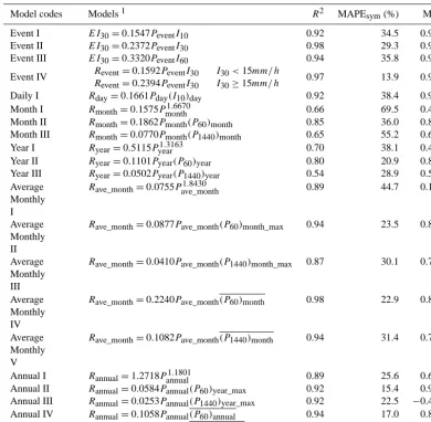
uti-Table 4. Models calibrated in this study and their prediction capabilities determined using the validation stations – the symmetric mean absolute percentage errors, MAPEsym, and Nash–Sutcliffe model efficiencies, ME.
Model codes Models1 R2 MAPEsym(%) ME
Event I EI30=0.1547PeventI10 0.92 34.5 0.91
Event II EI30=0.2372PeventI30 0.98 29.3 0.98
Event III EI30=0.3320PeventI60 0.94 35.8 0.96
Event IV Revent=0.1592PeventI30 I30<15mm/ h Revent=0.2394PeventI30 I30≥15mm/ h
0.97 13.9 0.98
Daily I Rday=0.1661Pday(I10)day 0.92 38.4 0.91
Month I Rmonth=0.1575Pmonth1.6670 0.66 69.5 0.48
Month II Rmonth=0.1862Pmonth(P60)month 0.85 36.0 0.88
Month III Rmonth=0.0770Pmonth(P1440)month 0.65 55.2 0.69
Year I Ryear=0.5115Pyear1.3163 0.70 38.1 0.48
Year II Ryear=0.1101Pyear(P60)year 0.80 20.9 0.84
Year III Ryear=0.0502Pyear(P1440)year 0.54 28.9 0.59
Average Monthly I
Rave_month=0.0755Pave_month1.8430 0.89 44.7 0.17
Average Monthly II
Rave_month=0.0877Pave_month(P60)month_max 0.94 23.5 0.88
Average Monthly III
Rave_month=0.0410Pave_month(P1440)month_max 0.87 30.1 0.73
Average Monthly IV
Rave_month=0.2240Pave_month(P60)month 0.98 22.9 0.88
Average Monthly V
Rave_month=0.1082Pave_month(P1440)month 0.94 31.4 0.79
Annual I Rannual=1.2718Pannual1.1801 0.89 25.6 0.63
Annual II Rannual=0.0584Pannual(P60)year_max 0.92 15.4 0.91
Annual III Rannual=0.0253Pannual(P1440)year_max 0.92 22.5 −0.44
Annual IV Rannual=0.1058Pannual(P60)annual 0.94 17.0 0.88
Annual V Rannual=0.0492Pannual(P1440)annual 0.92 18.2 0.91
1Parameters of models for power-law models, includingα
1,β1,α2,β2,α3,β3,α4,β4,α5,β5, were solved by pooling data from 11
stations together. Parameters for average annual-scale models, includingλ15,λ16,λ17,λ18, were calculated by fitting data from all
calibration stations and for the remainder they were the average values of parameters for the 11 calibration stations.2R2is the coefficient
of determination.
lized (P1440)year_max, the maximum of (P1440)yearvalues for
each year over the entire period of record.
Tables 3 and 4 show the models only evaluated for the ero-sivity temporal scale that corresponds to the input data res-olution. For example, the event-based models are only eval-uated on the basis of events modeled. We also evaleval-uated the models at the aggregate scale. For example,EI30 estimated
from event-based models were summed up to month and year values, in order to evaluate if fine temporal resolution data also improve the accuracy of aggregate erosivity measures (Table 6). Two important facts emerge. First, when the mod-els are applied at the aggregated scale their predictions get better. Secondly, the models that use fine resolution of input data predict better for the same erosivity timescale compared
to models using coarser resolution input data. This has im-portant implications for model applications.
3.3 Seasonal variations of erosivity
[image:8.612.103.493.97.479.2]0 100 200 300 400 500 600 700 0
3000 6000 9000 12000
Monthly rainfall (mm)
M
on
th
ly
R
(M
J m
m
h
a
-1 hr -1 )
(a) Month I
Rmonth=0.1575*Pmonth1.6670, r2=0.66
0 400 800 1200 1600 2000 2400 0
4000 8000 12000 16000
Yearly rainfall (mm)
Y
ea
rly
R
(M
J mm
h
a
-1 hr -1 a -1 )
(b) Year I
Ryear=0.5115*Pyear1.3163, r2=0.70
0 50 100 150 200 250 0
600 1200 1800 2400
Average monthly rainfall (mm)
A
ver
age m
ont
hl
y R
(M
J m
m
ha
-1 hr
-1 ) (c) Average Monthly I
Ravemonth=0.0755*Pavemonth1.8430 , r2=0.89
0 200 400 600 800 100012001400 0
2000 4000 6000 8000
Annual rainfall (mm)
A
nnual
R
(M
J m
m
ha
-1 hr -1 a -1 )
(d) Annual I
[image:9.612.116.482.66.345.2]Rannual=1.2718*Pannual1.1801, r2=0.89
Figure 2. Scatterplots for power-law models using rainfall amount: (a) Month I, (b) Year I, (c) Average Monthly I, and (d) Annual I, based on the 11 calibration stations.
Table 5. Validation station-averaged symmetric mean absolute percentage errors (MAPEsym) and Nash–Sutcliffe model efficiency
coeffi-cients (ME) forRmonthby Month I,Ryearby Year I andRave_monthby Average Monthly I models for seven validation stations and statistics
on event rainfall amount and eventEI30.
Station name Rmonthby Month I Ryearby Year I Rave_monthby Average Percent of EI30/P
Monthly I erosive amount (%)
MAPEsym ME MAPEsym ME MAPEsym ME
Tonghe 70.2 0.73 30.9 0.47 29.5 0.93 71.2 4.8
Yangcheng 65.5 0.31 27.1 0.55 16.4 0.96 81.7 4.2
Miyun 52.0 0.71 45.1 −0.06 37.6 0.88 82.8 7.8
Xichang 77.5 0.47 45.4 −0.15 57.2 0.09 76.9 4.1
Huangshi 70.1 0.65 24.5 0.63 46.1 0.73 86.5 5.7
Tengchong 83.4 −2.01 66.6 −7.51 68.3 −6.98 71.9 3.6
Changting 52.0 0.54 20.9 0.26 35.2 0.30 88.4 6.1
Mean1 67.2 0.20 37.2 −0.83 41.5 −0.44 79.9 5.2
Mean2 62.0 0.59 29.7 0.37 38.7 0.60 82.1 5.7
1Averaged value for seven validation stations.2Averaged value for five validation stations except Xichang and Tengchong.
Seasonal variations by monthly and average monthly mod-els (Fig. 3) and yearly variations by month and year modmod-els (Fig. 4) were demonstrated using Tonghe and Tengchong sta-tions. Month I and Average Monthly I captured the general seasonal pattern for the Tonghe station (Fig. 3a and c), but the simulated peak value of monthlyRwas in July for the Teng-chong station, which was not consistent with observation.
[image:9.612.89.505.435.598.2]to-Table 6. MAPEsymfor the models when used to estimate longer timescales of erosivity.
Model Models Event and Month Avg. Year Annual
codes Daily monthly
Event I EI30=0.1547PeventI10 34.5 29.0 20.4 16.4 12.0
Event II EI30=0.2372PeventI30 29.3 24.2 16.0 11.4 9.1
Event III EI30=0.3320PeventI60 35.8 28.5 15.1 10.8 6.2
Event IV Revent=0.1592PeventI30 I30<15 mm h
−1 Revent=0.2394PeventI30 I30≥15 mm h−1
13.9 11.0 7.0 6.4 4.7
Daily I Rday=0.1661Pday(I10)day 38.4 29.2 19.6 16.2 11.7
Month I Rmonth=0.1575Pmonth1.6670 69.5 46.7 39.4 28.7
Month II Rmonth=0.1862Pmonth(P60)month 36.0 19.9 18.6 13.1
Month III Rmonth=0.0770Pmonth(P1440)month 55.2 26.7 24.8 12.3
Year I Ryear=0.5115Pyear1.3163 38.1 23.5
Year II Ryear=0.1101Pyear(P60)year 20.9 14.3
Year III Ryear=0.0502Pyear(P1440)year 28.8 17.3
0 2 4 6 8 10 12 0
10 20 30 40 50
60 (a) Tonghe from month models
Month
A
ve
ra
ge
m
ont
hl
y R
(%
) Observation Month I Month II Month III
0 2 4 6 8 10 12 0
10 20 30 40 50
60 (c) Tonghe from average monthly models
Month
A
ve
ra
ge
m
ont
hl
y R
(%
) Observation Average Monthly I Average Monthly II Average Monthly III
0 2 4 6 8 10 12 0
10 20 30
40 (b) Tengchong from month models
Month
A
ve
ra
ge
m
ont
hl
y R
(%
) Observation Month I Month II Month III
0 2 4 6 8 10 12 0
10 20 30
40(d) Tengchong from average monthly models
Month
A
ve
ra
ge
m
ont
hl
y R
(%
[image:10.612.81.511.87.256.2]) Observation Average Monthly I Average Monthly II Average Monthly III
Figure 3. Comparisons of average monthlyRvalues between observation values calculated using 1 min resolution rainfall data and estimated
values using month models (a, b) and average monthly models (c, d) for the Tonghe and Tengchong stations.
tal rainfall at those stations were lower (71.9 and 76.9 %, re-spectively), suggesting that more events occurred with small amount totals that do not generate soil loss (Table 5); and (2) the ratio for eventEI30to event rainfall amountP was lower
(3.6 and 4.1, respectively), inferring that rainfall intensity and erosivity generated by per amount of rainfall were both less than that of the other stations (Table 5). This result was consistent with that of Nel et al. (2013), which demonstrated that two models using annual average rainfall and average
[image:10.612.111.482.272.552.2]19600 1970 1980 1990 2000 2000
4000
6000 (a) Tonghe from month models
Year
Y
ea
rly
R
(M
J mm h
a
-1 h -1 a
-1 ) Observation
Month I Month II Month III
19600 1970 1980 1990 2000 2000
4000
6000 (c) Tonghe from year models
Year
Y
ea
rly
R
(M
J mm h
a
-1 h -1 a
-1 ) Observation
Year I Year II Year III
1960 1970 1980 1990 2000 1000
5000 9000 13000
17000 (b) Tengchong from month models
Year
Y
ea
rly
R
(M
J mm h
a
-1 h -1 a
-1 ) Observation
Month I Month II Month III
1960 1970 1980 1990 2000 1000
5000 9000 13000
17000 (d) Tengchong from year models
Year
Y
ea
rly
R
(M
J mm h
a
-1 h -1 a
-1 ) Observation
[image:11.612.102.498.64.335.2]Year I Year II Year III
Figure 4. Comparison of yearlyRvalues between observation values calculated using 1 min resolution rainfall data and estimated values
using month models (a, b) and year models (c, d) for the Tonghe and Tengchong stations. The years without marks were ineffective years.
3.4 Evaluation of models from previous research with current models
Generally speaking, the finer the resolution of input data for models, the better was the performance of the model for es-timating at the same temporal erosivity scale. For example, the models with daily rainfall amount and daily maximum 60 or 10 min amount as inputs performed better than mod-els with only daily rainfall amount as input. Similarly, results from models with maximum 60 min rainfall amount (Month II, Year II, Average Monthly IV, and Annual IV) were gener-ally better than those with maximum daily rainfall amount (Month III, Year III, Average Monthly V, and Annual V; Fig. 5).
Wang et al. (1995) used a combination of event rainfall amount Pevent and I10 for event-scale models. The model
using the I10 data was divided into two categories, with
a threshold of 10 mm h−1, performed best among the four
models compared (Table 3). That model had similar perfor-mance with Event IV in this study (Table 4), which also di-vided the data by a rainfall-intensity threshold.
There were three kinds of daily-scale models, according to the number and type of inputs required. Two models used daily rainfall amount (Zhang et al., 2002b; Xie et al., 2015), two models used daily rainfall amount and daily maximum 10 min intensity (Xie et al., 2001 and Daily I), and one model used daily rainfall amount and daily maximum 60 min
inten-sity (Xie et al., 2015). The model with daily rainfall amount as input in Xie et al. (2015) performed better than that of Zhang et al. (2002b) (Table 3). Daily I, which used daily rainfall amount and daily maximum 10 min intensity as in-puts in this study, performed better than the model in Xie et al. (2001). Models with an additional daily 10 or 60 min in-tensity index performed better than those with only a total rainfall amount (Tables 3 and 4).
There were generally four groups of models for month, year, average monthly, and annual-scale models. The first group used linear regression (Sun et al., 1990; Wu, 1994; Zhou et al., 1995) or a power-law function (Zhang and Fu, 2003; Month I, Year I, Average Monthly I, and Annual I) with only rainfall amount as input, so that the data required were relatively easy to collect. Models by Sun et al. (1990), Wu (1994) and Zhou et al. (1995), when they were used to estimate the monthly scale of R, had MAPEsym values of
86.7, 60.2 and 67.3 % and ME of−0.63, 0.57 and 0.35, re-spectively (Table 3). When they were used to estimate an-nual scale ofR, there was a tendency of underestimation, especially for the stations with larger erosivity (Fig. 5a, b). Four models by Zhang and Fu (2003) overestimated the R factor, with MAPEsymvarying between 34.6 and 60.8 % and
0 4000 8000 12000 16000 0
4000 8000 12000
16000 (a) Month models
Observed R (MJ mm ha-1 hr-1 a-1)
Es
tima
te
d R
(M
J mm h
a
-1 hr -1 a -1 )
Wu Zhou Month I Month II Month III
0 4000 8000 12000 16000 0
4000 8000 12000
16000 (b) Year models
Observed R (MJ mm ha-1 hr-1 a-1)
Es
tima
te
d R
(M
J mm h
a
-1 hr -1 a -1 )
Sun Wang Zhang Year I Year II Year III
0 4000 8000 12000 16000 0
4000 8000 12000
16000 (c) Average monthly models
Observed R (MJ mm ha-1 hr-1 a-1)
Es
tima
te
d R
(M
J mm h
a
-1 hr -1 a -1 )
Average Monthly I Average Monthly IV Average Monthly V
0 4000 8000 12000 16000 0
4000 8000 12000
16000 (d) Annual models
Observed R (MJ mm ha-1 hr-1 a-1)
Es
tima
te
d R
(M
J mm h
a
-1 hr -1 a -1 )
[image:12.612.114.483.66.344.2]Wang Zhang Annual I Annual IV Annual V
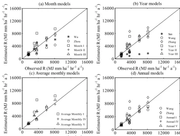
Figure 5. Comparisons of the estimatedRfactor value calculated based on (a) month, (b) year, (c) average monthly, and (d) average annual
models using 1 min resolution data for the seven independent validation stations. Month models included models in Wu (1994), Zhou et al. (1995), and Month I, II, and III from this study. Year models included models from Sun et al. (1990), Wang et al. (1995; the one with MAPEsymof 20.3 %), Zhang and Fu (2003), and Year I, II, and III from this study. Average monthly models included models from Average
Monthly I, II, and III from this study. Average annual models included models from Wang et al. (1995; the one with MAPEsymof 13.2 %),
Zhang and Fu (2003; the one with MAPEsymof 34.6 %), and Annual I, II, and III from this study.
using average annual rainfall as input (Table 3), which was consistent with the findings of Yu and Rosewell (1996). The power-law models in this study, including Month I, Year I, Average Monthly I, and Annual I, tended to overestimate the
R factor for the stations with larger erosivity (Fig. 5).
The second group of models (Wang et al., 1995; Month II, Year II, Average Monthly IV, Annual IV) used linear re-gression with rainfall amount (total rainfall or total rainfall with daily rainfall no less than 10 mm) and maximum 60 min rainfall as inputs. All these seven models generated statisti-cally significant results, with MAPEsymfor R with timescale
intended for the model ranging from 13.2 to 36.0 % and ME from 0.79 to 0.91 (Tables 3 and 4; Fig. 5).
The third group used linear regression with rainfall amount and maximum daily rainfall as inputs (Month III, Year III, Average Monthly V, Annual V), which generated reason-able results (Treason-able 4) and a slightly overestimated annualR (Fig. 5). Overall they did not perform as well as did the mod-els in the second group (Table 4).
The fourth group (Wang et al., 1995) used a combina-tion of three indices, including rainfall amount, maximum 60 min rainfall amount, and maximum daily rainfall amount as inputs and generated good simulation results; however,
there was no improvement compared with the two models by Wang et al. (1995) in the second group (Table 3). 3.5 Applications and recommendations
The results of this study provide a multitude of options for dealing with the problem of variations in available tempo-ral resolutions of rainfall data from across the world for de-veloping erosivity maps and databases. We present a series of 21 potential equations for use in estimating erosivity at timescales from event to average annual using input data res-olution ranging from maximum 10 min rainfall intensity to average annual rainfall amount. Of the 21 equations we can recommend the use of 17. Equations Month I, Year I, and Average Monthly I, which use only total rainfall amounts for the respective timescales, all had low ME values and poor prediction capability (Table 4). Annual III, which is a lin-ear function of average annual rainfall and the maximum daily precipitation over the recording period, performed very poorly, with a negative ME value (Table 4).
gave slightly better results than using I60 or I10. However,
we also found that using equations with the finest data reso-lution possible, and aggregating or summing results for finer erosivity timescales, gave the best results (Table 6). In other words, if one were interested in average annual erosivity, but had rainfall data available for using the Daily I model, then results are better using the Daily I model and summing re-sults over the period of data record rather than using Annual I–V models. It is also evident that predictions of erosivity using Daily I improve as the timescale increases. In other words, the predictions of average annual erosivity calculated by summing the daily values from Daily I give a higher level of fit than when using Daily I to estimate daily erosivity (Ta-ble 6).
Models in this study performed better or similar to mod-els from previous research given the same rainfall data in-puts based on these independent validation data (Tables 4 and 5). Models from previous research had higher symmet-ric mean absolute percentage errors, MAPEsym, and lower Nash–Sutcliffe model efficiencies, ME, with the exception of models for event, year, and average annual timescales by Wang et al. (1995), which had similar MAPEsym and ME compared to the models in this study.
Much attention has been given to monitoring the erosion process and its controlling factors at various spatiotempo-ral scales (Poesen et al., 2003). Characteristics of topogra-phy and soils are usually relatively constant in the timescales of interest, whereas rainfall erosivity and vegetation vary greatly. Therefore, soil erosion monitoring work is often mainly focused on the dynamics of rainfall erosivity and veg-etation rather than soil and topography (Vrieling et al, 2014). Different timescales of erosivity are required in areas with different resolutions of rainfall data availability. Models pro-vided in this study have potential to play important roles in the soil erosion monitoring framework in terms of quantify-ing the temporal dynamics and changes in rainfall erosivity.
Acknowledgements. The authors would like to thank the Hei-longjiang, Shanxi, Shaanxi, Beijing, Sichuan, Hubei, Fujian, and Yunnan Meteorological Bureaus for supplying rainfall data and the three anonymous reviewers for their valuable and constructive comments. This work was supported by the National Natural Science Foundation of China (no. 41301281) and the China Scholarship Council. USDA is an equal opportunity provider and employer.
Edited by: N. Romano
References
Angulo-Martínez, M. and Beguería, S.: Trends in rainfall erosivity in NE Spain at annual, seasonal and daily scales, 1955–2006, Hydrol. Earth Syst. Sci., 16, 3551–3559, doi:10.5194/hess-16-3551-2012, 2012.
Armstrong, J. S.: Long-range forecasting: From crystal ball to com-puter, 2nd Edn., Wiley, New York, 1985.
Arnoldus, H. M. J.: Methodology used to determine the maximum potential average annual soil loss due to sheet and rill erosion in Morocco, FAO Soils Bull., 34, 39–51, 1977.
Bonilla, C. A. and Vidal, K. L.: Rainfall erosivity in Central Chile, J. Hydrol., 410, 126–133, 2011.
Brown, L. C. and Foster, G. R.: Storm erosivity using idealized in-tensity distributions, Trans. ASABE., 30, 379–386, 1987. Capolongo, D., Diodato, N., Mannaerts, C. M., and Piccarreta, M.:
Analyzing temporal changes in climate erosivity using a simpli-fied rainfall erosivity model in Basilicata (southern Italy), J. Hy-drol., 356, 119–130, 2008.
China Meteorological Administration (CMA): Specifications for surface meteorological observation, Meteorology Publishing House, Beijing, 2003.
Fan, J., Chen, Y., Yan, D., and Guo, F.: Characteristics of rainfall erosivity based on tropical rainfall measuring mission data in Ti-bet, China, J. Mountain Sci., 10, 1008–1017, 2013.
Ferro, V., Porto, P., and Yu, B.: A comparative study of rainfall ero-sivity estimation for southern Italy and southeastern Australia, Hydrolog. Sci. J., 44, 3–24, 1999.
Flanagan, D. C., Meyer, C. R., Yu, B., Scheele, D. L.: Evalua-tion and enhancement of the CLIGEN weather generator, in: Proceedings–Soil Erosion Research for the 21st Century, edited by: Ascough II, J. C. and Flanagan, D. C., American Society of Agricultural Engineers, St. Joeseph, 107–110, 2001.
Foster, G. R.: User’s Reference Guide: Revised Universal Soil Loss Equation (RUSLE2), US Department of Agriculture, Agricul-tural Research Service, Washington DC, 2004.
Fournier, F.: Climate et erosion; la relation entre lerosion du sol par leau et les precipitations atmospheriques, Universitaires de France, Paris, 1960.
Larionov, G. A.: Erosion and Wind Blown Soil. Moscow State Uni-versity Press, Moscow, 1993.
Laws, O. J. and Parsons, D. A.: The relation of drop size to intensity. Trans. AGU, 24, 452–460, 1943.
Liu, B. Y., Zhang, K. L., and Xie, Y.: An empirical soil loss equa-tion. in: Proceedings–Process of soil erosion and its environment effect (Vol. II), 12th international soil conservation organization conference, Tsinghua University Press, Beijing, 21–25, 2002. Liu, B. Y., Guo, S. Y., Li, Z. G., Xie, Y., Zhang, K. L., and Liu, X.
C.: Water erosion sample survey in China, Soil Water Conserv. China, 10, 26–34, 2013.
Lo, A., EI-Swaify, S. A., Dangler, E. W., and Shinshiro, L.: Effec-tiveness ofEI30as an erosivity index in Hawaii, in: Soil Erosion
and Conservation, edited by: EI-Swaify, S. A., Moldenhauer, W. C., and Lo, A., Soil Conservation Society of America, Ankeny, 384–392, 1985.
Ma, X., He, Y. D., Xu, J. C., Noordwijk, M. V., and Lu, X. X.: Spatial and temporal variation in rainfall erosivity in a Himalayan watershed. Catena, 121, 248–259, 2014.
Makridakis, S. and Hibon, M.: Evaluating accuracy (or error) mea-sures. Working paper, INSEAD, Fontainebleau, France, 1995. McGregor, K. C. and Mutchler, C. K.: Status of the R factor in north
McGregor, K. C., Bingner, R. L., Bowie, A. J., and Foster, G. R.: Erosivity index values for northern Mississippi, Trans. ASABE., 38, 1039–1047, 1995.
Nash, J. E. and Sutcliffe, J. V.: River flow forecasting through con-ceptual models, Part 1: A discussion of principles, J. Hydrol., 10, 282–290, 1970.
Nearing, M. A. and Bradford, J. M.: Single waterdrop splash de-tachment and mechanical properties of soils, Soil Sci. Soc. Am. J., 49, 547–552, 1985.
Nel, W., Anderson, R. L., Sumner, P. D., Boojhawon, R., Rughoop-uth, S. D. D. V., and DunpRughoop-uth, B. H. J.: Temporal sensitivity anal-ysis of erosivity estimations in a high rainfall tropical island en-vironment, Geogr. Ann. A, 95, 337–343, 2013.
Nicks, A. D. and Lane, L. J.: Weather Generator, in: USDA-Water Erosion Prediction project: Hillslope profile and watershed model documentation, edited by: Flanagan, D. C. and Nearing, M. A., NSERL Report No. 10. USDA-ARS National Soil Ero-sion Research Laboratory, West Lafayette, IN, 2.1–2.22, 1995. Oliveira, P. T. S., Wendland, E., and Nearing, M. A.: Rainfall
ero-sivity in Brazil: A review, Catena, 100, 139–147, 2012. Panagos, P., Ballabio, C., Borrelli, P., Meusburger, K., Klikc, A.,
Rousseva, S., Perˇcec Tadi´c., M., Michaelides, S., Hrabalíková, M., Olsen, P., Aalto, J., Lakatos, M., Rymszewicz, A., Du-mitrescu, A., Beguería, S., and Alewell C.: Rainfall erosivity in Europe, Sci. Total Environ., 511, 801–814, 2015.
Poesen, J., Nachtergaele, J., Verstraeten, G., and Valentin, C.: Gully erosion and environmental change: importance and research needs, Catena, 50, 91–133, 2003.
Ramos, M. C. and Duran, B.: Assessment of rainfall erosivity and its spatial and temporal variabilities: Case study of the Penedès area (NE Spain), Catena, 123, 135–147, 2014.
Renard, K. G. and Freimund, J. R.: Using monthly precipitation data to estimate the R- factor in the revised USLE, J. Hydrol., 15, 287–306, 1994.
Renard, K. G., Foster, G. R., Weesies, G. A., McCool, D. K. and Yoder, D. C.: Predicting soil erosion by water. Agriculture Hand-book 703, US Department of Agriculture, Agricultural Research Service, Washington DC, 1997.
Richardson, C. W., Foster, G. R., and Wright, D. A.: Estimation of erosion index from daily rainfall amount, T. ASAE, 26, 153–156, 1983.
Roose, E.: Erosion et ruissellement en Afrique de louest-vingt an-nees de mesures en petites parcelles experimentales. Pour faire face à ce problème préoccupant, I’ORSTOM et les Instituts Travaux et Documents de I’ORSTOM, No. 78, O.R.S.T.O.M, Paris, 1977.
Sadeghi, S. H. R. and Tavangar, S.: Development of stational models for estimation of rainfall erosivity factor in different timescales, Nat. Hazards, 77, 429–443, 2015.
Sadeghi, S. H. R., Moatamednia, M., and Behzadfar, M.: Spatial and Temporal Variations in the Rainfall Erosivity Factor in Iran, J. Agr. Sci. Tech., 13, 451–464, 2011.
Sanchez-Moreno, J. F., Mannaerts, C. M., and Jetten, V.: Rainfall erosivity mapping for Santiago island, Cape Verde, Geoderma, 217, 74–82, 2014.
Schwertmann, U., Vogl, W., and Kainz, M.: Bodenerosion durch Wasser, Eugen Ulmer GmbH & Co., Stuttgart, 1990.
Seber, G. A. F. and Wild, C. J.: Nonlinear Regression. John Wiley & Sons, Inc., Hoboken, 2003.
Snedecor, G. W. and Cochran, W. G.: Statistical Methods, 12th Edn., The Iowa State University Press, Ames, 1989.
Sun, B. P., Zhao, Y. N., and Qi, S.: Application of USLE in loessial gully hill area. Memoir of NISWC, Academia Sinica and Min-istry of Water Conservancy, Yangling, 12, 50–59, 1990. Vrieling, A., Sterk, G., and de Jong, S. M.: Satellite-based
estima-tion of rainfall erosivity for Africa. J. Hydrol., 395, 235–241, 2010.
Vrieling, A., Hoedjes, J. C. B., and van der Velde, M.: Towards large-scale monitoring of soil erosion in Africa: Accounting for the dynamics of rainfall erosivity, Global Planet. Change, 115, 33–43, 2014.
Wang, B. M., Lu, Y. P., and Zhang, Q.: The color scanning digitizing processing system of precipitation autographic record paper, J. Appl. Meteor. Sci., 15, 737–744, 2004.
Wang, W. Z.: Index of ranfall erosivity (r) in loess area. Soil Water Conserv, China, 12, 34–40, 1987.
Wang, W. Z., Jiao, J. Y., and Hao, X. P.: Distribution of rainfall erosivity R value in China, J. Soil Water Conserv., 9, 5–18, 1995. Wischmeier, W. H. and Smith, D. D.: Rainfall energy and its rela-tionship to soil loss, T. Am. Geophys. Union, 39, 285–291, 1958. Wischmeier, W. H. and Smith, D. D.: Predicting rainfall-erosion losses from cropland east of the Rocky Mountains, Agriculture Handbook 282, US Department of Agricultural Research Ser-vice, Agricultural Research SerSer-vice, Washington DC, 1965. Wischmeier, W. H. and Smith, D. D.: Predicting rainfall erosion
losses: A guide to conservation planning, Agriculture Handbook 537, US Department of Agricultural, Agricultural Research Ser-vice, Washington DC, 1978.
Wu, S. Y.: Simplified method on calculation of runoff erosion force in Dabieshan mountainous area and its temporal and spatial dis-tribution, Soil Water Conserv. China, 4, 1–13, 1994.
Xie Y., Zhang, W. B., and Liu, B. Y.: Rainfall erosivity estimation using daily rainfall amount and intensity, Bull. Soil Water Con-serv., 6, 53–56, 2001.
Xie Y., Liu B. Y., and Nearing M. A.: Practical thresholds for sepa-rating erosive and non-erosive storms, T. ASAE, 45, 1843–1847, 2002.
Xie, Y., Yin, S. Q., Liu, B. Y., Nearing, A. M., and Zhao, Y.: Models for estimating daily rainfall erosivity, J. Hydrol., in review, 2015. Yin, S. Q., Xie, Y., Nearing, M. A., and Wang, C. G.: Estimation of rainfall erosivity using 5- to 60-minute fixed-interval rainfall data from China, Catena, 70, 306–312, 2007.
Yu, B.: Rainfall erosivity and its estimation for Australia’s tropics, Aust. J. Soil Res., 36, 143–165, 1998.
Yu, B. and Rosewell, C. J.: A robust estimator of the R-factor for the universal soil loss equation, T. ASAE, 39, 559–561, 1996. Zhang, W. B. and Fu, J. S.: Rainfall erosivity estimation under
dif-ferent rainfall amount, Resour. Sci., 25, 35–41, 2003.
Zhang, W. B., Xie, Y., and Liu, B. Y.: Estimation of rainfall erosivity using rainfall amount and rainfall intensity, Geogr. Res., 21, 384– 390, 2002a.
Zhang, W. B., Xie, Y., and Liu, B. Y.: Rainfall erosivity estima-tion using daily rainfall amounts, Sci. Geogr. Sin., 22, 705–711, 2002b.