Molecular Dynamics Simulations Towards The Understanding of the Cis Trans Isomerization of Proline As A Conformational Switch For The Regulation of Biological Processes

ScholarWorks @ Georgia State University

ScholarWorks @ Georgia State University

Chemistry Dissertations Department of Chemistry

8-12-2014

“Coarse Grained" Bead Modeling of Macromolecules Transport in

“Coarse Grained" Bead Modeling of Macromolecules Transport in

Free Solution and in a Gel

Free Solution and in a Gel

Follow this and additional works at: https://scholarworks.gsu.edu/chemistry_diss

Recommended Citation Recommended Citation

Wu, Hengfu, "“Coarse Grained" Bead Modeling of Macromolecules Transport in Free Solution and in a Gel." Dissertation, Georgia State University, 2014.

https://scholarworks.gsu.edu/chemistry_diss/98

This Dissertation is brought to you for free and open access by the Department of Chemistry at ScholarWorks @ Georgia State University. It has been accepted for inclusion in Chemistry Dissertations by an authorized

administrator of ScholarWorks @ Georgia State University. For more information, please contact

FREE SOLUTION AND IN A GEL

by

HENGFU WU

Under the Direction of Dr. Stuart Allison

ABSTRACT

The modeling of transport behavior of charged particles carried out in our laboratory is

based on classical continuum electro kinetic theory. It is applied to a variety of systems from

small electrolyte ions to macromolecules including peptides, DNA and nanoparticles. Systems

range from weakly charged particles to highly charged ones. Transport properties studied include

conductance, electrophoresis, and diffusion.

In this dissertation, the conductance of polyvalent electrolytes ions is studied both by a

coarse-grained continuum primitive model is developed and used to characterize the titration and

electrical conductance behavior of aqueous solutions of fullerene hexa-malonic acid, which is a

highly charged electrolyte with an absolute valence charge as high as 12.

Free solution electrophoresis is closely related to conductance and a coarse-grained bead

modeling methodology, BMM, developed in the Allison’s laboratory starting in 2006, is

generalized to characterize peptide systems with respect to the charge, conformation, and

possibly specific interactions with components of the BGE. For weakly charged peptides, the

electrostatic potential is treated at the level of linear Poisson-Boltzmann equation, which predicts

the electrophoretic mobility with considerable accuracy [S. Allison, H. Pei, U. Twahir, H. Wu, J.

Sep. Sci., 2010, 33(16):2430-2438], but fails for highly charged systems. A new nonlinear

Poisson-Boltzmann, NLPB-BM procedure is developed and applied to the free solution

electrophoretic mobility of low molecular mass oligolysines. The difficulty of highly charged

systems is twofold: more complex handeling of electrostatics and accounting for the relaxation

effect. Both issues are addressed in this dissertation.

A related problem we investigated deals with the retarding influence of a gel on the

rotational motion of a macromolecule. This is investigated within the framework of the Effective

Medium (EM) model and is applied to examine the electric birefringence decay of a 622 base

pair DNA fragment in an agarose gel. Modeling is also compared with experiment.

FREE SOLUTION AND IN A GEL

by

HENGFU WU

A Dissertation Submitted in Partial Fulfillment of the Requirements for the Degree of

Doctor of Philosophy

in the College of Arts and Sciences

Georgia State University

Copyright by Hengfu Wu

FREE SOLUTION AND IN A GEL

by

HENGFU WU

Committee Chair: Stuart Allison

Committee: Donald Hamelberg Jenny Yang

Electronic Version Approved:

Office of Graduate Studies

College of Arts and Sciences

Georgia State University

DEDICATION

ACKNOWLEDGEMENTS

The work described in this Dissertation has been accomplished with the assistance and

support of many people. First and foremost, I would like to express my sincere appreciation and

gratitude to my advisor, Dr. Stuart Allison. He taught me how to start academic pursuits from the

very beginning. From him I have learned a lot, particulary in the area of Computational

Chemistry. Without his encouragement and help, I could not have completed my PhD work.

I would also like to thank my committee members: Dr. Donald Hamelberg, and Dr. Jenny

Yang for their helpful advice on my Dissertation, and I would also like to thank Dr. Dabney

White Dixon for her great concern for me and her help to me all the time.

I would like to thank the Department of Chemistry at Georgia State University for

offering me the opportunity to pursue the Ph.D. degree, for offering great classes and the

opportunity to teach undergraduate students in laboratories and tutorials. All of these provided

me good training in academic matters. Specially, I would like to thank Dr. Stuart Allison, Dr.

Markus Germann, Dr. David Wilson, Dr. Jerry Smith, Dr. Dabney Dixon, Dr. Kathryn Grant, Dr.

Jenny Yang, Dr. Donald Hamelberg, Dr. Ivaylo Nikolaev Ivanov and Dr. Aimin Liu for their

interesting classes. I would also like to thank my previous group members, Hongxia Pei, Umar

Twahir, and other group members, and my friends for discussions and help. Last but not least, I

would like to express my gratitude to my family. Thanks to my parents' great love and support

and my sister, Sheling Hao's encouragement all the time. Special thanks go to my wife, Kun

TABLE OF CONTENTS

ACKNOWLEDGEMENTS ... iv

LIST OF TABLES ... x

LIST OF FIGURES ... xi

1 INTRODUCTION……….1

1.1 Brief Introduction of Electrophoresis………...1

1.2 The Modeling Methodology of Transport of Charged Praticles ... 3

1.3 Outline of the Dissertation ... 5

2 CONDUCTIVITY AND ELECTROPHORETIC MOBILITY OF DILUTE IONIC SOLUTIONS ... 7

2.1 Introduction ... 7

2.2 Modeling ... 9

2.2.1 Conductance and Mobility of Small Ion Electrolytes ... 9

2.2.2 Mobility of Large Spherical Ions ... 17

2.2.3 Analysis of Conductance Data ... 27

2.3 Results ... 30

2.3.1 Application to KCl ... 30

2.3.2 Application to MgCl2 and LaCl3 ... 33

2.4 Discussion ... 37

3 ROTATIONAL DIFFUSION OF MACROMOLECULES AND

NANOPARTICLES MODELED AS NON-OVERLAPPING BEAD ARRAYS IN

AN EFFECTIVE MEDIUM ... 42

3.1 Introduction ... 42

3.2 Results and Discussion ... 43

3.2.1 Transport Theory of Bead Arrays in an Effective Medium ... 43

3.2.2 Modeling the Rotation of Linear Macromolecules as Strings of Identical, but Non-Overlapping Beads ... 52

3.2.3 End-over-End Rotation of Rods ... 54

3.3 Experimental section: Rotational Relaxation of DNA in a Dilute Agarose Gel ... 56

3.4 Conclusions ... 59

4 MODELING THE ELECTROPHORESIS OF HIGHLY CHARGED PEPTIDES: APPLICATION TO OLIGOLYSINES ... 61

4.1 Introduction ... 61

4.2 Materials and Methods ... 62

4.2.1 Experiments and Modeling Backgroud ... 62

4.2.2 Accounting for Electrostatics at the Level of the Nonlinear PB Equation 63 4.2.3 Charge State, the Relaxation Correction, and the IISM Binding Model ... 71

4.3 Results ... 74

4.5 Concluding Remarks ... 76

5 COARSE GRAINED MODELING OF THE TITRATION AND CONDUCTANCE BEHAVIOUR OF AQUEOUS FULLERENE HEXAMALONIC ACID(FHMA) SOLUTIONS ... 81

5.1 Introduction ... 81

5.2 Methods ... 84

5.3 Results ... 86

5.3.1 pK1 and pK2 for Models A, B, and C (no counterion binding) ... 86

5.3.2 Inclusion of Na+ Specific Binding for Models A and C ... 88

5.3.3 Conductance of FHMA in the Presence of Ca2+ at 25 _ºC ... 89

5.3.4 Distributions of FHMA Species with pH...89

5.4 Discussion ... 93

5.5 Concluding Remarks ... 93

REFERENCES ... 101

APPENDICES ... 111

LIST OF TABLES

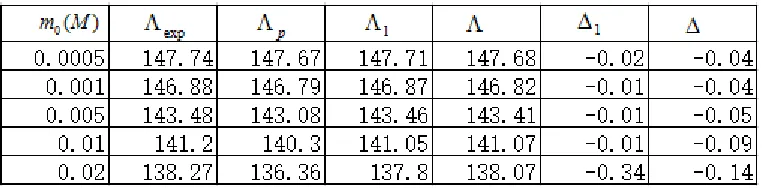
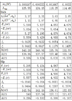
Table 2.1 Comparison of KCl equivalent conductance between experiment and samll ion theory

... 32

Table 2.2 Comparison of equivalent conductance between experiment and large ion theory ... 32

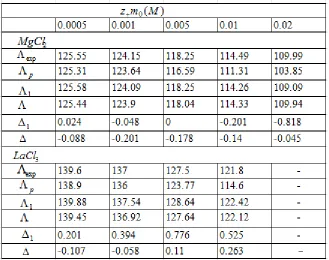
Table 2.3 Conductance data for MgCl2 and LaCl3 (small ion model) ... 35

Table 2.4 Conductance/mobility data on MgCl2 (large ion model) ... 36

Table 2.5 Conductance/mobility data on LaCl3 (large ion model) ... 37

Table 4.1 “Large ion” relaxation coefficients ... 78

LIST OF FIGURES

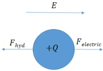
Figure 1.1 A spherical charged particle in free solution with applied electric field ... 1

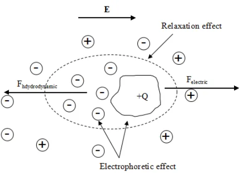
Figure 1.2 An irregular shaped charged particle in neutral solution surrounded by electrolyte ions in the presence of electric field ... 2

Figure 2.1 Experimental and model equivalent conductances for KCl, MgCl2, and LaCl3 ... 40

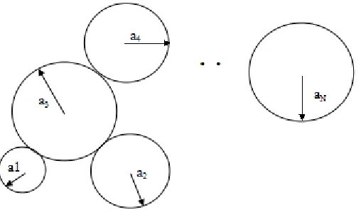
Figure 3.1 Array of N non overlapping beads ... 44

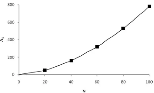
Figure 3.2 Λ1 for a right circular cylinder and linear string of touching beads versus length ... 56

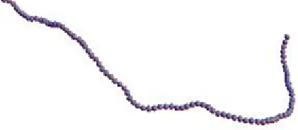
Figure 3.3 A 88 subunit discrete wormlike chain ... 58

Figure 3.4 Model and experimental Λ1 values for 622 bp DNA as a function of gel concentraion ... 59

Figure 4.1 Subdivision of space exterior to the bead array ... 79

Figure 4.2 Dependence of µ on n for experiment and “nonbinding models” of oligolysines ... 80

Figure 4.3 Dependence of µ on n for experiment and IISM binding models of oligolysines ... 81

Figure 5.1 Structure of FHMA... 83

Figure 5.2 Conductivity, κ (in 10-4 1/(ohm m)), versus αn of FHMA and Models A, B, and C with no counterion binding at 25 °C, cx = 1.15 x 10-4 M...89

Figure 5.3 Titration curve (pH versus αn) of FHMA and Model A with pK1 = 1,8, pK2 = 4.2, and pKB = -1.4 at 25 °C cx = 1.15 x 10-4 M. ...90

Figure 5.5 Equivalent Conductance, Λ (in 10-4 m2/(ohm mole)) of FHMA versus c for Model A

and experiment at pH = 6 and 25 °C where the counterion is Ca+2...91

Figure 5.6 Ion Charge Distributions and Extent of Counterion Binding in Model FHMA...93

CHAPTER 1

INTRODUCTION

1.1 Brief Introduction of Electrophoresis

Charged particles, under the influence of electric fields, migrate toward the electrode with

the opposite charge, and this phenomena is called electrophoresis. Electrophoretic mobility

depends on particle size and charge, or the ratio of charge over size. The higher the ratio, the

faster the particle moves subjected to the same electric field for a period of time. Particles of

different size and charge travel different distances. Electrophoretic techniques have been widely

used in chemistry, molecular biology, microbiology, and colloid science, etc. Macromolecules,

like proteins, peptides and nucleocapsids, as well as small molecules, like amino acid,

nucleotides, and organic ions can migrate in an electric field. The simplest possible case is

illustrated in Figure 1-1. When immersed in a neutral solvent of viscosity, η, applied electric

field of strength E, a spherical particles of charge +Q, and radius a, migrates at a constant

velocity due to the influence of two forces.

Figure 1-1: A spherical charged particle in free solution with applied electric field

Feletric is the electrical force acting on the charged particles due to the electric field, and Fhdy is the

hydrodynamic force acting on the particle due to the surrounding viscous solvent. The magnitude

) 1 1 ( Feletric =QE −

) 2 1 (

6 −

= av

F_hyd πη

Where v is the particle moving velocity, Q is the effective charge of particle, E is the

electric field strength, η is the solution viscosity, and a is the hydrodynamic radius of particle.

Under steady state, both forces equal to each other,

) 3 1 (

6 −

= av

E Q πη

Rearrange equation (1-3) to derive the electrophoretic mobility, µ

) 4 1 (

6 −

= =

a Q E v

η π µ

The main problem of electrophoresis theory is to determine both forces for model

systems, which, however, are not as simple as a spherical particles in the idealized system

described above. In actual cases, the presence of the background electrolyte ions affects the

migration of “guest” particles. As shown in Figure 1-2, an irregular shaped particle migrates in a

free solution with applied electric field, E, and the other ions of the background electrolyte must

be accounted for.

For the case shown in Figure 1-2, the positively charged particle is surrounded by

negatively charged electrolyte ions, which form an ion atmosphere, called double layer around

the “guest” particle. Under the influence of an electric field, positively charged ions move toward

the cathode, and negative ions toward the anode. During the migration, the counter ions, which

migrate in the opposite direction from the guest ion, cause a hydrodynamic drag force to act on

the guest particle, slowing down its motion. This effect is called the “electrophoretic effect”.

Also, the surrounding ion atmosphere is distorted under the influence of an external electric field,

which gives rise to another force on the guest particle. This effect is called the “relaxation effect”.

The “relaxation effect” can be ignored for weakly charged particles, but becomes significant for

highly charged particles. Both effects slow down the migration of particles, and make the

theoretical treatment of electrophoresis complicated and difficult.

1.2 The Modeling Methodologies of the Transport of Charged Particles

One of the early successes of atomic scale continuum transport modeling concerned the

electrical conductance of dilute solutions of strong electrolytes [1-3]. It is based on equilibrium

theory of strong electrolytes by Debye and Huckel [4], and the electrolyte ions were modeled as

point charges, and then extended to account for the finite size of the ions, and also for higher

electrolyte concentrations [5-7]. It was subsequently extended to general electrolyte solutions

with an arbitrary number of ions of arbitrary valence [8]. Such an approach is collectively called

the “small ion” model. Despite the successes of the “small ion” model, few applications were

made to electrolyte solutions containing polyvalent ions or mixtures of electrolytes containing

more complex ionic species. One shortcoming of the “small ion” model is that electrostatics are

treated at the level of linear Poisson-Boltzmann equation, and this makes it applicable to only

binary electrolytes and also polyvalent salts for which experimental conductance data is available.

This is the subject of Chapter 2.

A transport phenomenon closely related to electrical conductivity is the free solution

electrophoretic mobility. Free solution electrophoresis and related techniques play a vital role in

separation and characterization of peptides as discussed in a number of reviews [9-14].

Understanding the electrophoresis at the fundamental level of continuum electrodynamics and

hydrodynamics can provide information about peptide charge and possibly conformation [13-20].

The peptide mobility in the limit of low concentration is influenced by a variety of factors,

including the composition of BGE, temperature, solvent viscosity, and pH. These factors are

critical in defining optimal experimental conditions for separation. Generally, two different

approaches have emerged in modeling peptide mobility, µ. The first is based on the work of

Offord [22], which is semi empirical.The mobility is written [9-13, 17-19, 21,23]

) 5 1 (

1 ₋

≅ _α

µ

M Z c

or

) 6 1 ( )

log( 3

2 + ₋

α

M c Z c

Where, Z is the effective peptide charge, M the molecular mass, c1, c2, c3 and α are

empirical constants, depending on solvent, temperature, and BGE. However, these models fail

for highly charged or hydrophobic peptides [21]. The second approach is grounded on continuum

electro hydrodynamic theory, which has its origin in the electrophoresis and conductivity of

spherical ions [3, 5, 24-30]. This continuum theory accounts in more detail for the distribution of

the peptide charge and its primary and secondary structure [21, 31, 32]. It enables the

shape and charge are defined. Continuum theory has also been applied to long [33] and finite [34]

rods, axi-symmetric ellipsoids [35-37] and rigid particles of arbitrary shape and charge

distribution [38-40]. To deal with the problem of flexible structures, a bead modeling

methodology (BMM) has been developed and applied to peptides [41-45]

Until recently, the applications were largely restricted to weakly charged peptides, such

as oligoglycines [42]. By “weakly charged”, we mean the absolute surface or “ζ” potential does

not exceed about 25 mV [46], or equivalently, the electrophoretic mobility does not exceed

approximately 0.20 (cm2/(kV s)) [47]. For large or highly charged particles, a “large ion” model,

grounded on very similar continuum electro-hydrodynamic principles, is relevant since it

accounts for the “relaxation effect” [26-30, 48]. The “relaxation effect” becomes significant for

highly chared particles including pepetides and it is essential to accurately account for its

influence on electrophoretic mobility. Careful accounting of the relaxation effect greatly

improves agreement between modeling and experiment, as illustrated in Chapter 4.

1.3: Outline of the Dissertation

In this Dissertation, the transport behavior of small binary electrolytes ions, DNA

molecules, highly charged peptides, and nanoparticles are modeled based on classic electro

kinetic theory. The effects from BGE, pH, and temperature on the electrophoretic mobility are

examined. Chapter 2 examines the equivalent conductance of binary electrolytes with two

complimentary continuum theories of electro kinetic transport. The main objective is to bridge

the gap between the “small ion” and “large ion” models by modifying the O’Brien and White

(“large particle” model) procedure. In Chapter 3, the retarding influence of a gel on the rotational

motion of a macromolecules is investigated within the framework of the Effective Medium (EM)

birefringence. This chapter does not involve the electrokinetics, but the closely related problem

of continuum hydrodynamics. In chapter 4, bead modeling methodology is generalized to treat

electrostatic at the level of the nonlinear Poisson-Boltzmann equation, which makes it more

applicable to the important class of highly charged macroions and highly charged peptides in

particular. In chapter 5, the “coarse-grained” continuum primitive model is developed and used

to characterize the titration and electric conductance behavior of aqueous solutions of fullerene

hexa malonic acid, FHMA. This involves numerical solution of the non-linear

CHAPTER 2

CONDUCTIVITY AND ELECTROPHORETIC MOBILITY OF DILUTE IONIC

SOLUTIONS

2.1 Introduction

One of the early successes of atomic scale continuum transport modeling concerned the

electrical conductance of dilute solutions of strong electrolytes [1-3]. This work, in turn, was

grounded on equilibrium theory of strong electrolytes by Debye and Huckel [4]. The early theory,

which was restricted to very dilute solutions of ions modeled as point charges, was subsequently

extended to account for the finite size of the ions and also higher electrolyte concentrations [5-7].

For monovalent binary aqueous electrolyte solutions up to a concentration of about 0.10 mol/dm3

or M, experimental and model equivalent conductance are in excellent agreement [5-7] for

reasonable choices of model parameters. Refs. [5-7] are restricted to binary electrolytes. This

was subsequently extended to general electrolyte solutions made up of an arbitrary number of

ions of arbitrary valence [8]. In the present work, this approach shall collectively be called the

‘‘small ion” model. Despite the successes of the ‘‘small ion” model, there have been few

attempts to apply it directly to electrolyte solutions containing polyvalent ions or mixtures of

electrolytes containing more complex ionic species. One of its shortcomings is that electrostatics

are treated at the level of the linear Poisson– Boltzmann equation which limits it to weakly

charged particles. The theory has been generalized to go beyond the use of the linear Poisson–

Boltzmann equation in representing the ionic potential of mean force [49,50].

A transport phenomenon closely related to electrical conductivity is the free solution

electrophoretic mobility. In recent years, capillary zone electrophoresis [9–14] has become a

51-53], organic anions [54, 55], proteins [40, 56, 57], and nanoparticles [58, 58]. Although the

conductance theories discussed in the previous paragraph [3,5–7] have been applied to mobility

studies of small and weakly charged ions [54, 55, 60, 61], they are not appropriate for large or

highly charged particles including nanoparticles [58, 59] or metal oxide colloidal particles [62].

For large and/or highly charged particles, there is a long established alternative that is grounded

on very similar continuum electro-hydrodynamic principles, but has its origin in the

electrophoresis of large colloidal particles [26-30, 48]. In this work, it shall be called the ‘‘large

ion” model. Of particular relevance to the ‘‘large ion” model is the numerical procedure of

O’Brien and White [30] that has come into widespread use and can be applied to the

electrophoresis of a spherical particle of arbitrary size containing a centrosymmetric charge

distribution of arbitrary net charge. One factor that may limit the application of the ‘‘large ion”

model to treat the mobility or conductivity of small ions is that it ignores the Brownian motion of

the ion of interest. This may only be a reasonable approximation if the ion of interest is much

larger than the ions comprising the surrounding electrolyte. The ‘‘small ion” model, on the other

hand does account for the Brownian motion of all ions present [3, 5-8, 49, 50].

The principle objective of the present work is to bridge the gap between the ‘‘small ion”

and ‘‘large ion” models discussed above by applying both to the conductivity of a number of

binary electrolytes for which experimental conductance data is available. Polyvalent salts shall

also be considered in order to test the models under conditions of larger ‘‘zeta” potential. In the

course of this work, it has been necessary to modify the O’Brien and White (‘‘large particle”

model) procedure in three ways. The first is to include an ‘‘ion free” layer of solvent just outside

the surface of hydrodynamic shear. In addition to the distance of hydrodynamic shear from the

concerns hydrodynamic boundary conditions. In both ‘‘small ion” and ‘‘large ion” models,

hydrodynamic boundary conditions have been handled somewhat differently and it is important

to consider how this influences the results. Currently, ‘‘stick” boundary conditions are employed

in the ‘‘large ion” model, and this means the particle velocity and fluid velocity match at the

surface of hydrodynamic shear. In addition to the conventional ‘‘stick” hydrodynamic boundary

conditions, we also consider ‘‘slip”. As shall be shown, both ‘‘stick” and ‘‘slip” models are

capable of explaining the experimental conductance data equally well for about the

same a_ex values, but different a_j values must be chosen on the basis of limiting ionic

conductivities. Third, although the ‘‘large ion” model does not account explicitly for the

Brownian motion of the central ion of interest, we present a simple way of doing so that involves

adding a correction term to the mobile ion mobilities. When this is done, the ‘‘small ion” and

‘‘large ion” model conductivities with the same or similar model parameters are comparable with

each other and yield excellent agreement with experiment.

2.1 Modeling

2.2.1 Conductance and Mobility of Small Ion Electrolytes

The original Onsager [2] and Onsager–Fuoss [3] theory treats the equivalent conductivity,

Λ, or electrophoretic mobility of ionic species j, of dilute strong electrolyte;

) 1 2 ( )

( _{0 0}

0− Λ + −

Λ =

Λ_p α β m

In Eq. (2-1), the ‘‘p” subscript denotes the original Onsager–Fuoss model mobility, Λ0 is

the equivalent conductance of the solution in limit of zero ionic strength, α is the ‘‘relaxation

electrolyte in moles/dm3 or M if it did not dissociate into ions. The physical basis of α is ion

relaxation, the distortion of the ion atmosphere around a particular ion from equilibrium due to

the imposition of an electric and/or flow field. The physical basis of β is the additional

hydrodynamic backflow produced in the vicinity of a particular ion produced by the presence of

nearby ions. The coefficients α and β depend on: temperature, T, the properties of the solvent

including relative dielectric constant,ε_r, and viscosity, η, and the valence charges of the ionic

species present in solution, {zj}. They are, however, independent of ionic size. Ionic size,

however, does enter through Λ0 or equivalently, the electrophoretic mobility of individual ions in

the limit of zero ionic strength, I. Underlying Eq. (2-1) is a model in which the ions are treated as

point charges. The Onsager–Fuoss, OF, theory [2,3] starts with a general equation of continuity

which specifies the concentration of ions of one species in the vicinity of ions of other species in

an electrolyte solution which has reached a steady state under the influence of a weak, constant

external electric field, e0. Account is taken of the Brownian motion of the various ionic species

of which an arbitrary number may be present. Electrostatics are treated at the level of the linear

Poisson–Boltzmann equation. This is true not only for the ‘‘point ion” model discussed here, but

the more general finite ion case considered at the end of this section. For the ‘‘point ion” model,

the boundary conditions on the fluid velocity are that it remain finite at the center of an ion and

vanish, on average, at a large distance away from it. The general OF mobility expression of an

ionic species can be written [3]

) 2 2 ( )

( ₂

0

) ( 0

1

0 − ∑ + −

= ∞

= c r B z I

z

B _j

n

n j n j

j j

j µ µ

µ

(

)

2 1/2

2 / 3 6 2 / 3 0 3 1 − × = = − − M T RT N F B r r AV ε ε ε π ) 4 2 ( ) sec ( ) ( 10 275 . 4 ) ( 6 2 2 / 1 2 2 / 1 6 2 / 1 0 2 2 − × = = − − M V m T RT N F B r r

AV η ε

ε ε πη

In the present work, SI units shall be followed for the most part, but g in Eq. (2-4) is in

centipoise and I is in moles/ dm3 = M. For the remaining terms, F is the Faraday constant

(=9.645 *104 C/mole), NAv is Avogadro number, ε0 is the permittivity of free space, R is the gas

constant, and other quantities (except for c_nandr_j(n)) have been described in the previous

paragraph. Also, the physical basis of the B1 term in Eq. (2-2) is ion relaxation and the physical

basis of the B2 term is the electrophoretic effect.

Consider a single strong electrolyte, A_aB_b or binary electrolyte, that undergoes complete

dissociation according to

) 5 2

( −

+

→ z+ z−

b

aB aA bB

A

Where a andb, z₊and z₋are stoichiometries and valences of the two ions. If m0 is the

initial concentration of undissociated electrolyte, then the condition of electrical neutrality

requires ) 6 2 ( 0 0

0z+ +bm z− = − am And ) 7 2 ( )) ( 2 ( ) ( 2 0 2 0 2 2

0 + = − = −

= + _{+ −}

−

+ z z m m

az bz

az m

The conductivity, Λ, of a solution of this strong electrolyte can be written ) 8 2 ( | | | | | | 0 0 0 0 0 0 0 0 − Λ = − = + = Λ + Λ = + = + − + + − − + + − − + + − + z am Fz am Fz bm Fz am z bm z am bm am K µ µ µ µ λ λ

The λ_j terms appearing in the first equality on the right hand side of Eq. (2-8) are molar

conductivities of specific ions. TheΛ_jvalues appearing in the second equality on the right hand

side of Eq. (2-8) correspond to equivalent conductivities of specific ions. Most, but not all, of the

specific ion conductivities reported in the modern literature and in handbooks areΛ_j’s and in SI

units are in S m2/mole or m2/ (ohm mole). The third equality follows from the relationship

between equivalent ionic conductance and ion mobility, which will be positive for + ions and

negative for - ions, Λ_j =F|µ_j |. The fourth equality follows from the electro neutrality

condition, Eq. (2-6). The fifth equality gives the equivalent conductance of the binary

electrolyte,Λ. Dividing various equalities on the right hand side of Eq. (2-8) by am₀z₊gives

) 9 2 ( |) | | (| ) ( − = + − = Λ + Λ =

Λ _{+ −} F µ₊ µ₋ F µ₊ µ₋

For a strong binary electrolyte of the formAaBb, the ‘‘relaxation” term in Eq. (2-2)

according to the OF theory can be written (3)

If the binary electrolyte is also a symmetric electrolyte (|z+| = |z_|), then q = 1/2. Using

Eqs. (2-2), (2-7), and (2-10) in (2-9), we have for a general binary electrolyte

) 12 2 ( |)] | | (| ) (

[ _{1 0 0 3 0}

0 − Λ +Λ + + −

Λ =

Λ B ₊ S_{+ −} S₋ B z₊ z₋ φ m

) 13 2 ( 0 0

0 =Λ +Λ −

Λ _{+ −}

) 14 2 ( ) ( ) ( 4125 . 0 2 / 1 2 2 / 1 2

3 = = −

M mole ohm m T FB B r ε η

It should be emphasized that g in Eq. (2-14) is in centipoise. Comparing Eqs. (2-12) with

(2-1), and equating Λ withΛ_p, we can now identify the relaxation and electrophoresis

coefficients, ) 15 2 ( ) ( 0 0 0 1 ₋ Λ Λ + Λ

= + + − − φ

α B S S

) 16 2 ( |) | | (|

3 + −

= + − φ

β B z z

The expression for αsimplifies further within the framework of the OF theory. From Eq.

(2-10) we have S+ = S_ = S and Eq. (2-15) then reduces to

) 17 2

( −

=β φ

α S

In order to make contact with different relaxation theories, however, we have chosen to

distinguish the relaxation terms for the different ions, Sj, defined by Eq. (2-10).

For an electrolyte consisting of more than two ionic species, the relaxation effect is more

complex than discussed in the previous paragraph, which is strictly valid only for a binary

of distinct ions. Assume we have N ions present and let mj denote the concentration (in M) of

species j. For this more general case, the Sj terms are given by the first equality on the right hand

side of Eq. (2-10). We have [3]

) 25 2 ( ) ( ) 24 2 ( | | / ) 23 2 ( ) 22 2 ( ) 1 )( / ( ) ( ) 21 2 ( ) 2 ( ) 20 2 ( ) 1 ( ) 1 2 3 ( ) 19 2 ( 3535534 . 0 ) 18 2 ( 2928932 . 0 2 / ) 2 2 ( 1 0 1 2 2 1 1 ) 0 ( ) 0 ( ) 1 ( ) ( 1 1 0 − + + + = − Λ = − = − − = = − ⋅ − = − > − = − − = − = − =

∑

∑

∑

∑

k i j

j j k i k k ij ij j j j N k k k

j j j

j N

k k k

N k k k j j j n n n n w w w u w w w u H z w z m z m u w w u z u z r r r I H r n n c c c c δ

In Eq. (2-21), r(0) is a N by 1 column vector and H and I are N by N matrices. Also,I is

the identity matrix and dij is the Kronecker delta. In general, it is necessary to solve for Sj

iteratively. One begins by determining r(0) from Eq. (2-22) and known input parameters. The

same input parameters are used to determine the components ofH. Then Eq. (2-21) is used to

generate r(n) for higher order terms in n. These along with cn defined by Eqs. (2-18) - (2-20) are

used in Eq. (2-10) to compute Sj. In most cases, the series converges rapidly with n. Despite its

apparent complexity, this procedure is actually quite simple and straightforward to implement

in a computer program or an Excel spreadsheet, which will be shared with interested

investigators upon request to the corresponding author. In terms of the dimensionless

) 26 2 ( )

( _{1 0 2}

0− + −

= _j B _j S_j B z_j I

j µ µ

µ

In the 1950s, Fuoss and Onsager generalized this theory to extend its range of validity to

terms of order in 1 0

m electrolyte concentration and also account, to lowest order, for the finite

sizes of the ions [6,7]. This work was restricted to binary electrolytes and specific applications in

this and subsequent work [63-65] were further restricted to monovalent (binary) electrolytes.

Quint and Vaillard [8] did generalize this to an arbitrary electrolyte and included terms to order

2 / 3 0

m although some contributions at the level of 3/2 0

m are missing [66]. In these studies [6–8, 63–

66] a single ion exclusion distance,a_ex, is defined and the assumption is made that the

center-to-center distance, r, between any two ions cannot be smaller thana_ex. The assumption is also made

that the normal component of the relative fluid velocity vanishes at r =a_ex (see Eq. (2-3, 2-4) of

(2-7)). Closely related work was also carried out by Pitts [5] on symmetric binary electrolytes,

but the assumption was made that the relative fluid velocity as a whole, and not just the normal

component, vanishes at r =aex. Within the framework of the more general Fuoss–Onsager theory

[6, 7], the equivalent conductance of a binary electrolyte can be written

) 27 2 ( ) 1 ( − − Λ =

Λ nr ξ

) 28 2 ( ) 1 ( 0

0 − + −

Λ =

Λnr β m καex

) 29 2 ( 0 − Β = φ m

) 31 2 ( )

1

( ₀

0 ' 3 2

1

0 _Λ −

∆ + ∆ + ∆ −

=α m β m

ξ

The term Λ_nris the equivalent conductance in the absence of ion relaxation, n denotes the

relaxation correction, and j is the Debye–Huckel screening parameter. In Eq. (2-31), the

terms∆₁,∆₂, and ' 3

∆ represent higher order correction terms and depend on concentration to

leading order 1/2 0

m . Explicit expressions are given in Section 7 of Ref. [7] specific to symmetric

binary electrolytes. More general expressions (making minor corrections for sign errors) can be

deduced from equations in Section 6 of Ref. [7] for general binary electrolytes. In subsequent

work by Fuoss and coworkers, additional corrections were made to∆₂, and ∆'₃[63-65, 67].

However, these changes were minor and do not alter the relaxation corrections significantly. In

addition, expressions not limited to binary electrolytes can be found in references [8, 66] and

include terms to order 3/2 0

m . Since the 1957 paper by Fuoss and Onsager [7] carries out the most

thorough comparison between theoretical and experimental conductance and subsequent

applications are mostly restricted to monovalent binary electrolytes, we shall use the equations

from the 1957 paper [7] in the present work when considering the ‘‘small ion” model. The

‘‘small ion” theory pioneered by Fuoss and Onsager [2, 3] remains in widespread use to this day

not only for fully dissociated electrolytes, but undissociated electrolytes as well [68]. With few

exceptions [66], the over-whelming majority of applications involve symmetric binary

electrolytes [68-70]. The limiting assumptions of the ‘‘small ion” theory are: (1) solvent and

mobile ions are treated as a continuum, (2) electrostatics are described by the linear Poisson–

Boltzmann equation, (3) a single ion exclusion distance,a_ex, is included in modeling, (4) κa_exis

consider a simpler model that includes finite ion size effects in Λ_nras given by Eq. (2-28), but

restricts the relaxation term to 1/2 0

m and this allows us to ignore∆₁,∆₂, and ' 3

∆ altogether. Define

) 32 2 ( )

1

( ₀

1 =Λ − −

Λ _nr α m

As demonstrated in the main body of this work, Eq. (2-32) works almost as well as Eq.

(2-27) for binary electrolytes for m0 ≤0.005 M.

Finally, consider the ion electrophoretic mobilities within the framework of the

Onsager-Fuoss theory restricted to a binary electrolyte. We can write

) 33 2 ( )

1 (

, − −

= jnr j

j µ ξ

µ

) 34 2 ( )

1 (

0 2

0

,nr = j −Β Ζj + ex −

j µ φ m κα

µ

Where ξj is the same for both ions and the j subscript is omitted in Eq. (2-27) and (2-31).

As Eq. (2-31) shows, higher order concentration effects (via the∆₁,∆₂, and∆'₃ terms) can be

accounted for in binary electrolytes. However, it would be useful if we could also consider

ternary and higher order electrolyte solutions. This would be relevant if we were interested in the

mobility of a ‘‘guest” ion in the presence of a binary electrolyte, for example. Eq. (2-26) makes it

possible to consider such cases, where the relaxation term depends on the particular ion and we

can write

) 35 2 (

1 Ι −

Β ≅ Sj

ξ

) 36 2 ( 2

1 2 ₋

=

Ι

∑

κ κ κ

Where Sj is given by the first term on the right hand side of Eq. (2-10) and the sum in Eq.

(2-36) extends over all ions present in solution. For ternary and higher order electrolyte

solutions, we can approximate nj appearing in Eq. (2-33) with Eq. (2-35). This is equivalent to

ignoring terms higher than order I1/2 in the relaxation correction. The same approximation is

made in arriving at Eq. (2-32) for the conductivity of a binary electrolyte and Eq. (2-32)

therefore gives us a way of determining how accurate this approximation is in specific cases.

2.2.2 Mobility of Large Spherical Ions

It shall be assumed that our model particle is spherical and contains a centrosymmetric

charge distribution within a surface of hydrodynamic shear located at a distance r = afrom the

center of the particle. At the shear surface, ‘‘stick” or ‘‘slip” boundary conditions may prevail. In

the case of ‘‘stick”, it is assumed that fluid and particle velocities match at r =a. In the case of

‘‘slip” boundary conditions, it is assumed that only the outward normal component, n, of particle

and fluid velocities match at r =a. Also, ifσ_H denotes the hydrodynamic stress tensor of the

fluid, thenσ_H is parallel to n at the shear surface [71, 72]. Outside of the shear surface, the fluid

is treated as a hydrodynamic continuum that obeys the linearized Navier–Stokes and solvent

incompressibility equations.

) 37 2 (

2 _{−∇ =∇⋅ =− −}

∇ν ρ σ_Η s

η

) 38 2 (

0 −

= ⋅ ∇ ν

Where g is the fluid viscosity, v is the local fluid velocity, p is the local fluid pressure,

translating with velocity u*through a fluid that is at rest far from the particle, the solution of Eqs.

(2-37) and (2-38) for the fluid velocity,v0(r) can be written for r >a,

) 39 2 ( ) , ( ) (

0 _{=Τ ⋅} ∗ ₋

u r

r α

ν

Where for ‘‘stick” boundary conditions, the tensor,T(a,r) is [74]

) 40 2 ( ) 3 ( 4 ) ( 4 3 ) , ( ₃ 3 − − Ι + + Ι = Τ nn r nn r

r α α

α ) 41 2 ( 2 ₋

=rr r nn

And for "slip" boundary conditions,

) 42 2 ( ) ( 2 ) ,

( = Ι+ −

Τ nn

r a r a

In Eqs. (2-40) and (2-42), Idenotes the 3 by 3 identity matrix. The zero superscript on v0

is a reminder that this refers to the special case of an uncharged spherical particle.

Extending from r =a to r =aex, where aex is the ion exclusion distance, it is assumed that

no ions are present. In this region of the fluid adjacent to the particle, s=0. The fluid, however,

obeys Eqs. (2-37) and (2-38). For r >a_ex, the ion atmosphere is treated as a continuum. Let nj(r)

denote the local concentration of mobile ion species j in M and let zj denote the valence charge

of a single ion. The charge distribution,ρ(r), obeys the Poisson equation in general,

) 43 2 ( ) ( )) ( ) (

( ∇Ψ =− ₀ −

⋅

) 44 2 ( ) ( ) ( ) ( = +

∑

f r F z n r

r ρ

ρ

where ε₀ is the permittivity of free space,ε is the local relative dielectric constant, Ψ is

the electrodynamics potential, ρ_f is the fixed charge density (within the particle) and the sum in

Eq. (2-44) extends over all mobile ion species present. If it is assumed ε(r)=ε_i for r <aand

r

r ε

ε( )= for r >a, we also have the boundary condition

) 45 2 ( −       ∂ ∂ =       ∂ ∂ + − =

=α α

ψ ε ψ ε r r r i r r

Wherea_±denotes a point just outside or inside the particle surface. To proceed, we use

the notation and many of the protocols of O’Brien and White [30]. Due to the presence of a

constant external electric, e0, or flow field, the steady state electrodynamics potential is written

) 46 2 ( ) ( ) ( )

(r =ψ₀ r +ψ₁ r −e₀⋅r −

ψ

Where Ψ₀ is the local equilibrium electrostatic potential and Ψ₁is a perturbation potential

that vanishes far from the particle. The local ion densities are also perturbed from their

equilibrium values,n_j0(r), which are related to a new potential, φ_j(r), defined by

[

]

( )

( )

( = ₀ ( ( ) 1()) ≅ ₀ − + ₁ −

Β Τ + − Β T k r r ez r n e r n r

n_{j j} ezjφj r ψ r κ _{j j} φ_j ψ

) 48 2 ( )

( = −z y0(r) −

j jo j e m r n ) 49 2 ( ) ( ) ( 0

0 = −

Where kB is the Boltzmann constant. It is assumed that the perturbing electric or flow

field is sufficiently small that only terms to first order in those perturbing fields are significant.

This justifies the expansion of the exponential in Eq. (2-47). In addition to Eqs. (2-37), (2-38),

and (2-43), an ion

) 50 2 ( 0 − = ⋅ ∇ Jj

(

)

0

0 + ∇Φ + Τ −

=n Fz n D e R

J _{j j} ν _{j j j j}

Above, J_j is the local current density of species j and Dj is the translational diffusion

constant. Other quantities have been defined previously. The boundary condition on j arises as a

result of the constraint that mobile ions cannot approach the particle closer than a distancea_ex.

Setting J _j⋅n=0 in Eq. (2-51) then yields

( )

) 52 2 (

0⋅ −

− =       ∂ Φ ∂ = n e r r ex r j α

For a spherical particle, the solution of the equilibrium electrostatic potential is a special

case of Eq. (2-43). The reduced potential depends only on the distance from the center of the

particle, r.

For r >a,

( )

_{( )}

2 =− _Τ −

    

_∑

r ε ε κ ω

) 54 2 ( 1

0_{ =− −}

In Eq. (53), ω(r) is a step function which equals 0 for r < a_exand 1 for r >a_ex. In Eq.

(54), /(4 0 )

2

1 e Z ε εrkBTa

α = (dimensionless) and Z is the net valence charge of the particle. For a

weakly charged particle, the exponential in Eq. (53) can be expanded and the resulting linear

equation can be solved analytically. This is the linear Poisson–Boltzmann equation and the

reduced (dimensionless) potential for the present problem for r > a can be written

( )

(

)

The ‘‘LPB” superscript on y0 denotes the linear Poisson Boltzmann reduced potential. In

the present work, however, the general non-linear for of Eq. (2-53) is solved numerically subject

to the boundary condition imposed by Eq. (2-54).

For the nonequilibrium problem, we follow the strategy of carrying out two separate

transport cases (30). In Case 1, the particle is translated with constant velocity, u0, in a fluid that

is otherwise at rest. In Case 2, the particle is held stationary, but it is subjected to a constant

external electric field, e0. Although the potentials, ()(r)

i j

Φ are not spherically symmetric (the (i)

superscript has been added to distinguish the two transport cases), they can be written in terms of

related functions that are [30],

( )

_{( )}

_{( )}

Φ r b r

r

r ji i i

j φ

Where b(1) andb(2) =e₀. As discussed in detail previously [30], the coupled equations for

in the radial variable r. These are then solved numerically for the two transport cases. Let N

denote the number of mobile ions species present (which is two for a binary electrolyte). For

each transport case, N + 2 homogeneous and one inhomogeneous set of differential equations are

solved subject to different distant boundary conditions. The overall solution for Case 1 or 2 is

then taken to be a particular linear combination of the above mentioned N + 3 ‘‘distant” solutions

that satisfy appropriate boundary conditions at r = aex. The overall solution ofφj(r)for case i (i =

1 or 2), is

( )

_{( )}

_{( )}

0

− =

∑

=

−

κ

κ κ φ

φ_ji r d i _ji r

Where the sum over k extends over the inhomogeneous (k = 0) and different

homogeneous (j = 1 to N + 2) ‘‘distant” solutions, (ji k)(x) −

Φ is the k-th ‘‘distant” solution for

case i and ion j, and the (i)

k

d are the lin-ear coefficients that are determined from boundary

conditions on or near the particle as discussed later. For k = 0 or N + 1 or N + 2, the outer

boundary condition on (ji k)(x) −

Φ is set to 0. For k = 1 to N,

( )

_{( )}

₍

₎

2 ,

− >>

=

−

r r

r j

i

j κ

δ

φ κ κ

Where δ_j,k is the Kronecker delta.

The remaining two homogeneous ‘‘distant” solutions (k = N + 1 or N + 2) are associated

with the distant behavior of a scalar field, g(i )(r), from which the fluid velocity, v(1)(r), is

derived (30). It is defined by

( )

_{( )}

[

[

_{( )}

]

]

∞

i i i i

u b r g curl curl r

Whereb(i) is defined following Eq. (2-55) andu_∞(1) =−u₀, and u_∞(2) =0. The ‘‘distant”

solutions of g(i−j) are set to zero except for j = N+ 1

(−Ν+1)

_{( )}

r r g i

(−Ν+2)

_{( )}

r gi

The final expression for g(i)(r) can be written that is identical to Eq. (2-57) above with

) (i k

g − replacing φj(i−k). The d_k(i)coefficients appearing in Eq. (2-57) and an analogous relation

involving g(i)(r) and g(i-k)(r) are determined from ‘‘inner” boundary conditions. These are

discussed in reference [30] for the special case of ‘‘stick” boundary conditions when a =a_ex, but

the more general conditions of interest here must be handled differently. The boundary

conditions onφ(_ji)(r)follow from Eq. (2-52) and are simply (1)'( )₌0

ex j a

φ and (2)'( )₌0

ex j a

φ , where

the prime superscript denotes first derivative with respect to r. These are the same for both

‘‘stick” and ‘‘slip” hydrodynamic boundary conditions. The boundary conditions on g(i) are

evaluated at r = a and are different for ‘‘stick” and ‘‘slip”. For ‘‘stick”; g(j1)'(a)=−a/2,

2 / 1 ) ( ''

) 1

( ₌₋

a

gj and ( ) 0

''

) 2

( ₌

a

gj where the double prime denotes second derivative with respect

to r. For ‘‘slip”; careful analysis leads to the conditions:g(_j1)'(a)=−a/2, g(_j1)'''(a)=0, and

0 ) ( ''

) 2

( ₌

a

gj where the triple prime denotes third derivative with respect to r. With minor

modifications in Eq. (7.7) of reference [30] that incorporate these modified boundary conditions,

the (i)

k

taken to be the linear superposition of both Cases 1 and 2 fields that gives a net force exerted by

the particle on the fluid of zero [30].

At this point, it is appropriate to discuss how the results of Case 1 and Case 2 transport

studies can be used to obtain a general expression for the electrophoretic mobility, l, and then

reduce that to more recognizable forms in special cases. It is possible to obtain a general

expression of the electrophoretic mobility starting from the differential form of the Lorentz

reciprocal theorem [73, 74],

( )

(

)

(

)

) 62 2 (

0 0

0

0_{⋅ +∇⋅ ⋅ = ⋅ +∇⋅ ⋅ −}

Η Η

i i

i i

s

s ν ν σ ν ν σ

Where quantities with superscript (i) denote the actual fields around a charged spherical

particles (i = 1 or 2) and quantities with superscript 0 denote an arbitrary flow field that obeys

Eqs. (2-37) and (2-38) subject to appropriate hydrodynamic boundary conditions. For the

arbitrary fields, choose an uncharged sphere of radius a (same as the radius of our charged

particle) where v0 is given by Eqs. (2-39)– (2-42). Integrate Eq. (2-62) over the fluid domain,Ω,

exterior to a single isolated particle enclosed by surface Sp with outward normal (into the fluid),

n. Applying the divergence theorem yields

( ) ( ) ( )

) 63 2 (

0

0 _{⋅ =− ⋅ ⋅ + ⋅ Τ⋅ −}

⋅

−

_∫

_∫

_∫

Ω ∗ Η

Η ndS ndS u S dV

i i

S S

i σ ν σ

ν

ρ ρ

The total hydrodynamic force exerted by the particle on the fluid is

( )₌₋ ( )_{⋅ (2−64)}

∫

Η ndS

F

S i i

ρ

σ

And an entirely analogous expression can be written forFH0 . For ‘‘stick” boundary

the integral directly. For the ‘‘slip” case, first recognize that we can writeσH⋅n=(nn)⋅(σH⋅n).

Since the normal component of the fluid velocity matches that of the particle on Sp in the slip

case and since only the normal component contributes to the surface integrals, we can move

them out of the integrals also. The total force exerted by the particle on the fluid is the sum of

hydrodynamic and external (electrical) forces [30, 38, 75]

( ) ( ) ( )

∫

Τ =F + s dV (2−65)

F i i i

Using Eqs.(2-64) in Eq.(2-63)

( ) ( )

( )

) 66 2 (

0_{+ ⋅ Ι−Τ ⋅ −}

⋅ = ⋅

_∫

u i i i

In Eq. (2-66), u*is the velocity of our uncharged particle and u(i)the velocity of our

charged particle (Case 1 or 2). The external force term can be written [38, 75]

( )

(

)

2 0

0 ∇Φ + + Τ ∇ −

=

∑

∑

Using Eqs. (2-40), (2-42), (2-56)–(2-58), and (2-67) in (2-66), it is straightforward to

carry out the angular integrations. Also, the divergence theorem is applied to the second term on

the right hand side of Eq. (2-67). Without loss of generality, we can also assume the electric/

flow fields are along the x direction with (u*)=1 and only concern ourselves with the x

components of the overall forces. Eq. (2-66) can

( ) ( ) ( )

_∑

_{∑ ∫}

_{( )}

_{( )}

Τ = − + −

j i j j j j i j j j i i i r g r drn r z F d m z Fb f u F α π

π 4 (2 68)

3 4

0 2 0

( ) ( )

₍

₎

₍

₎

3 1 1 3 2 3 4 1 ' 2 1 2 1

1 + − − + − + −

  

  −

= i i

j i i j i i

j b h h b

r h h e

h

(

)

( )

0 = stick slip −

f πηα πηα

(

)

2 ; 4

3

1 = slip −

r stick r

h α α

(

)

(

)

4

1 3

2  −

    

= stick slip r

h α

( ) ( )

(

)

( ) ( )

(

)

4 3 4 1 1 0 2 2 −       − − − =

∑

∑

_{( )}

₍

₎

₍

₎

1 1 2 1 2 1 2 '

0 2 ₋         + − + − − +       −

=

_∫

j i j i j i

j h h

r h h h r drn

r δ φ φ

ρ

α

Eqs. (2-73) and (2-74) are general expressions for the mobility of a sphere and simplify in

limiting special cases.

Consider the special case where ion relaxation is neglected. This is a reasonable

approximation when the particle is weakly charged and the solution of the linear Poisson

Boltzmann equation, Eq. (2-55), is appropriate. Under these conditions, φ(_j1)=0, d(_j1)=0 ,

2 3 ) 2 ( /r ca j =

φ , d(_j2)=ca3, where c=(ε_r−ε_i)/(2ε_r+ε_i) All of the terms with superscript (1)

vanish in Eq. (2-73) and the d(_j2) term also drops out when we sum over j and impose the

condition of charge neutrality. Under these conditions, Eq. (2-73) reduces to

( )

(

)

3 2 3 4 4 2 1 3 3 1 0 2 0 0 −       − − + Ζ =

_∫

µ h h

The ‘‘nr” subscript denotes the ‘‘no relaxation” limiting case and ρ₀ is the equilibrium

charge density. For the ‘‘stick” and ‘‘slip” cases, Eq. (75) reduces to

( )

2 1 3 2 6 5 3 0 −               −       − + Ζ =

_∫

( )

2 1 3 2 4 3 0 −               − + Ζ =

_∫

It is straightforward to reduce these equations further. The charge

( )

_{( )}

) 78 2 (

2 ' ₀

' 0

0 ≅− Ι −

= − ΡΒ

∑

F r L j r y z j j j ρ

where =

∑

jmjzj

I' ( ' 2)/2 is the ionic strength in moles/m3, m'j is the ambient

concentration of species j in moles/m3, the exponential has been expanded and only the linear

term in y₀ has been retained. Furthermore, y0 has been approximated by its linear form given by

Eq. (2-55). Making use of Eqs. (2-55) and (2-78) in (2-76) and (2-77),

(

)

3 4 6 5 3 1 ' −                       −       − + Ι − Ζ =

_∫

(

)

3 4 4 3 1 ' −               − + Ι − Ζ =

_∫

The first term in brackets within the integrand on the right hand sides of Eqs. (2-79) and

(2-80) can be integrated directly and the c-terms can be reduced to exponential integrals. This

shall not be done here. Eqs. (2-79) and (2-80) provide a straightforward way of estimating the

weakly charged spherical particles. One example shall be given. Consider a=a_ex and c = 1/2,

Eq. (79) reduces to the Henry law mobility [26, 74]. The ratio of ‘‘slip” to ‘‘stick” mobilities

increases from 1.50, 1.56, 1.77, 2.07, and 3.30 for κa = 0, 0.12, 0.52, 1.10, and 3.39,

respectively.

2.2.3 Analysis of Conductance Data

Both the ‘‘small ion” and ‘‘large ion” theories described in the previous two sections

offer advantages and disadvantages and the principle objective of this work is to bridge these two

approaches and show how they complement each other. The greatest advantage of the ‘‘small

ion” approach is that it accounts for the Brownian motion of the principle ion of interest whereas

the ‘‘large ion” approach does not. The greatest advantage of the ‘‘large ion” approach is that it

accounts more accurately for the finite size of the ion and is not restricted to weakly charged

ions. (The ‘‘small ion” theories always employ the linearized form of the Poisson– Boltzmann

equation.) From Eq. (2-9), we have the relationship be-tween equivalent ionic conductance,Λ_j,

and absolute mobility, |µ_j|. In the limit of zero electrolyte, relaxation and electrophoretic, the

greatest advantage of the ‘‘small ion” approach is that it accounts for the Brownian motion of the

principle ion of interest whereas the ‘‘large ion” approach does not. The greatest advantage of

the ‘‘large ion” approach is that it accounts more accurately for the finite size of the ion and is

not restricted to weakly charged ions. (The ‘‘small ion” theories always employ the linearized

form of the Poisson– Boltzmann equation.) From Eq. (2-9), we have the relationship be-tween

equivalent ionic conductance,Λ_j, and absolute mobility,|µj |. In the limit of zero electrolyte,