Supply Chain Network Optimization by Considering
Cost and Service Level Goals
Mehmet Alegoz*
, Zehra Kamisli Ozturk
Department of Industrial Engineering, Anadolu University, 26555, Eskisehir, Turkey
Copyright©2018 by authors, all rights reserved. Authors agree that this article remains permanently open access under the terms of the Creative Commons Attribution License 4.0 International License
Abstract
In this study, we focus on designing the supply chain network of a company that sells households goods to its customers located in various cities of Turkey. Since the production plant of the company is fixed and cannot be changed, we divide the supply chain network design problem into two separate problems. In first problem, we focus on the network between the supplier and the production plant. This problem can be thought as a supplier selection problem and there are many qualitative and quantitative criteria, which affect this process. Therefore, we use Buckley’s Fuzzy AHP algorithm, which enables us to evaluate the suppliers according to all types of criteria. In second phase of the study, we focus on the supply chain network between the production plant, warehouses and customers and develop a multi objective mathematical model. Although, the proposed mathematical model gives optimal solution for our company data within a reasonable time, large size instances cannot be solved by using this model due to the complexity of problem. For this reason, we propose various metaheuristic approaches based on tabu search and compare the results with optimal solution. Computational results show that one of our approaches gives high quality results within a reasonable time. We conclude the study by discussing the numerical results and giving some future work suggestions to interested readers.Keywords
Multi-criteria Decision Making, Goal Programming, Tabu Search, Supply Chain Network Optimization1. Introduction
A supply chain is a set of facilities, supplies, customers, products and methods of controlling inventory, purchasing, and distribution [1].The chain links suppliers and customers, beginning with the production of raw material by a supplier, and ending with the consumption of a product by the customer [2]. Supply chain management
looks for the integration of a plant with its suppliers and its customers to be managed as a whole, and the coordination of all the input/output flows (materials, information and finances) so that products are produced and distributed at the right quantities, to the right locations, and at the right time [3].
In a supply chain, the flow of goods between a supplier and a customer passes through several echelons, and each echelon may consist of many facilities [2]. Efforts must be made to integrate suppliers, manufacturers, distributors, and customers, so that they will collaborate effectively with each other in the entire network [1]. By this context, a supply chain design problem comprises the decisions regarding the number and location of production facilities, the amount of capacity at each facility, the assignment of each market region to one or more locations, and supplier selection for sub-assemblies, components and materials [4]. In this study, we propose a two-phase cost and customer satisfaction oriented supply chain network design approach to deal with this problem.
The rest of the paper is organized as follows. In next section, we give the problem definition and literature review. In third and fourth sections, models related to first phase and second phase of study are given respectively. Finally, conclusion and future work suggestions are given in fifth section.
2. Problem Definition and Literature
Review
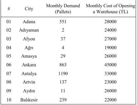
company does not plan to change the location of production plant. For this reason, the production plant must be thought as fixed. They want to open at most three warehouses. Monthly demand of each city and monthly cost of opening warehouse in each city are given only for ten cities in Table 1. The whole table that includes 81 cities is not given due to the space limit. Please note that monthly cost of opening a warehouse includes monthly renting and operating costs of a warehouse.
Table 1. Monthly Demand and Monthly Cost of Opening a Warehouse
# City Monthly Demand (Pallets) Monthly Cost of Opening a Warehouse (TL)
01 Adana 551 28000
02 Adıyaman 2 24000
03 Afyon 37 27000
04 Ağrı 4 19000
05 Amasya 29 26000
06 Ankara 863 45000
07 Antalya 1190 33000
08 Artvin 137 23000
09 Aydın 11 26000
10 Balıkesir 239 22000
The company wants to find answers to following questions.
Which supplier is best for them to work with? Where should be the warehouses opened? How many warehouses should be opened?
Which customers should be assigned to which warehouses?
What should be the monthly flow from each warehouse?
In order to answer these questions, we propose a two-phase supply chain network design approach. We divide the whole supply chain network design problem into two phases as it is seen in Figure 1. The first phase is designing the supply chain network between the supplier and production plant and the second phase is designing the supply chain network between the production plant, warehouses and customers.
We divide the problem into two phases because of three main reasons. These reasons are summarized below as follows.
(1) Since the production plant is located in Bilecik and it cannot be changed, the first phase and second phase are independent from each other. More specifically, for example, working with different suppliers does not affect the cost of second phase. Similarly, opening warehouses in different cities does not affect the cost of first phase. Briefly, these two phases can be modeled independently because of fixed location of production plant.
(2) In lots of studies, mathematical models are created to optimize the entire supply chain network. However, the suppliers should not be determined only according to one or a few objectives such as cost and service level. There are many other qualitative and quantitative criteria to evaluate the suppliers and it is necessary to put all of them into account to make an accurate selection. For this reason, in first phase, we use a multi-criteria supplier selection approach and in second phase, we develop a multi-objective mathematical model. (3) By dividing the problem into two phases, we
reduce the computational complexity. By this way, it may be possible to obtain the results within less CPU time.
There are numerous studies in literature about supplier selection problem. Some of them can be summarized as follows. Xia and Wu [5] focus on demand allocation in addition to supplier selection. They proposed an approach based on AHP improved by rough sets theory and multi-objective mixed integer programming. Zouggari and Benyoucef [6] proposed a simulation based fuzzy TOPSIS approach for supplier selection and demand allocation decisions. Ávila et al. [7] proposed a supplier’s selection model based on an empirical study. They used quality, finance, synergy, cost and manufacturing system as criteria in their study. Rajesh and Malliga [8] proposed an integrated supplier selection approach based on AHP and QFD to select the suppliers strategically. Cárdenas-Barrón et al. [9] developed an algorithm based on a reduce and optimize approach for the multi-product, multi-period supplier selection and lot sizing problem. Finally, Zarindast et al. [10] also focused on supplier selection problem and proposed a robust multi-objective global supplier selection model that works under demand and exchange rate uncertainties and takes care about price discounts.
[image:2.595.133.464.663.720.2]
In addition, many researchers focused on traditional or closed-loop supply chain network design problem and proposed single-objective or multi-objective models as follows. Wang et al. [11] focused on a rarely focused but important subject. They developed a green supply chain network model that takes care about the environment together with the total supply chain network cost. Pazhani et al. [12] proposed a multi objective model for supply chain network design problem. Their objectives are minimizing the total supply chain network cost and maximizing the service efficiency of warehouses and hybrid facilities. They used different variations of goal programming and compared the obtained results with each other. Hiremath et al. [13] developed a multi objective mathematical model for outbound logistics network design. Their objectives are minimizing the total supply chain network cost, maximizing the unit fill rate and maximizing the resource utilization of the facilities. Cárdenas-Barrón and Treviño-Garza [14] proposed a mathematical model in order to solve a multi-product, multi-period three-echelon supply chain network optimally.
Finally, there are also some metaheuristic approaches for the solution of supply chain network design problem. Yao and Hsu [15] used genetic algorithms for multi echelon supply chain network design problem. Easwaran and Üster [16] proposed an approach for closed loop supply chain network design problem, which consists of tabu search and Benders Decomposition. Costa et al. [17] proposed a new encoding and decoding approach for the supply chain network design problem. They used their proposed approach with genetic algorithms and they obtained high quality results. Cárdenas-Barrón et al. [18] focused on a three-layer supply chain consisting of supplier, manufacturer and retailer. They proposed an improved algorithm for this problem. Castillo-Villar and Herbert-Acero [19] focused on a rarely focused subject and they take care about the quality costs. They used simulated annealing and genetic algorithms to solve their supply
chain network model and compared the results obtained from both approaches.
Our study differs from the existing studies with following aspects. In this study, we focus on a real life problem and try to solve it with a two-phase approach. In first phase, suppliers are evaluated according to many qualitative and quantitative criteria with a fuzzy AHP approach. In second phase, a multi objective mathematical model is developed, which takes care about service level together with cost. For large size instances, we also propose hybrid metaheuristic approaches and compare their performances with each other.
3. Phase I: Supplier Selection
In this section, we focus on the first phase of the supply chain network, which is the network between the suppliers and production plant. As mentioned before, this problem can be thought as a supplier selection problem. Supplier selection is one of the most important subjects for a company to take care about. Since suppliers directly affect the performance of a company, it is essential to work with appropriate suppliers. This phase includes two important steps. First step is determining the criteria and their weights and second step is evaluating the suppliers according to those criteria and choosing one of them.
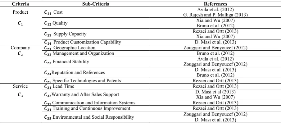
3.1. Determining the Criteria and Their Weights We use mainly two sources to determine the criteria. First one is the scientific publications about this problem and second one is expert opinions. When we collect and analyze the data obtained from both two sources, we see that expert opinions and scientific publications support each other. In the end, we determine three main criteria and fourteen sub-criteria, which affect the supplier selection process. These criteria and sub-criteria are given below in Table 2. A few references for each criterion are also provided.
Table 2. Criteria and Sub-Criteria
Criteria Sub-Criteria References
Product 𝑪𝑪𝟏𝟏𝟏𝟏 Cost G. Rajesh and P. Malliga (2013) Ávila et al. (2012)
𝑪𝑪𝟏𝟏 𝑪𝑪𝟏𝟏𝟏𝟏Quality Xia and Wu (2007) Bruno et al. (2012) 𝑪𝑪𝟏𝟏𝟏𝟏 Supply Capacity Rezaei and Ortt (2013) Xia and Wu (2007) 𝑪𝑪𝟏𝟏𝟏𝟏 Product Customization Capability D. Masi et al. (2013) Company 𝑪𝑪𝟏𝟏𝟏𝟏 Geographic Location Zouggari and Benyoucef (2012)
𝑪𝑪2 𝑪𝑪𝟏𝟏𝟏𝟏Management and Organization Bruno et al. (2012) 𝑪𝑪𝟏𝟏𝟏𝟏Financial Stability Zouggari and Benyoucef (2012) Ávila et al. (2012) 𝑪𝑪𝟏𝟏𝟏𝟏Reputation and References D. Masi et al. (2013) Bruno et al. (2012) 𝑪𝑪𝟏𝟏𝟐𝟐Specific Technologies and Patents Rezaei and Ortt (2013)
Service 𝑪𝑪𝟏𝟏𝟏𝟏Lead Time Rezaei and Ortt (2013)
[image:3.595.72.525.554.752.2]It can be seen in Table 2 that there are both qualitative and quantitative criteria, which affect the supplier selection process and all of them must be put into consideration in order to make a reliable analysis and obtain accurate results. For this purpose, we use type-2 fuzzy sets and Buckley’s fuzzy AHP algorithm.
Buckley’s fuzzy AHP algorithm mainly consists of seven important steps. We briefly explain these steps as follows. The reader may refer to Chen and Lee [23], Buckley [24] and Ozturk and Alegoz [25] for detailed information about the properties of type-2 fuzzy sets and Buckley’s fuzzy AHP algorithm.
Step 1: Consult experts for pairwise comparison of the critical success factors using linguistic variables.
Step 2: Examine the consistency of the pairwise comparison using crisp values proposed by Saaty [26].
Step 3: Construct type-2 fuzzy pairwise comparison matrix among all the criteria in the hierarchical structure as shown below.
�
1 𝛼𝛼��12
𝛼𝛼��21 1
⋯ 𝛼𝛼��1𝑛𝑛
⋯ 𝛼𝛼��2𝑛𝑛
⋯ ⋯
𝛼𝛼��𝑛𝑛1 𝛼𝛼��𝑛𝑛2
⋱ ⋯ ⋯ 1
� (1)
Step 4: Use geometric mean technique to define the fuzzy geometric mean as follows.
𝑟𝑟̃̃𝑖𝑖= (𝛼𝛼��𝑖𝑖1⊗𝛼𝛼��𝑖𝑖2⊗ … ⊗𝛼𝛼��𝑖𝑖𝑛𝑛)1/𝑛𝑛 (2)
Step 5: Calculate the fuzzy weights of each criterion by using the following equation.
𝑤𝑤��𝑖𝑖=𝑟𝑟̃̃𝑖𝑖⊗ (𝑟𝑟̃̃1⊕𝑟𝑟̃̃2⊕ … ⊕𝑟𝑟̃̃𝑛𝑛)−1 (3)
Step 6: Defuzzify the fuzzy number in order to calculate the weights of the criteria by using following equation.
𝑤𝑤𝑖𝑖′= 12�12∑4𝑖𝑖=1(𝑎𝑎𝑖𝑖𝐿𝐿+𝑎𝑎𝑖𝑖𝐿𝐿)� ⊗ 14�∑ �𝐻𝐻2𝑖𝑖=1 𝑖𝑖(𝐴𝐴𝐿𝐿) +
𝐻𝐻𝑖𝑖(𝐴𝐴𝑈𝑈)�� (4) Step 7: Use the following equation to normalize the crisp weights.
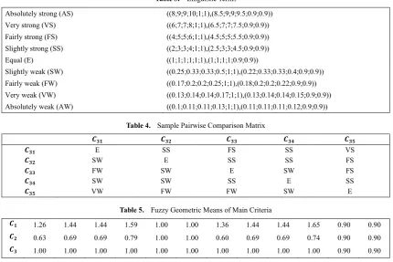
𝑤𝑤𝑖𝑖 = 𝑤𝑤𝑖𝑖′/∑𝑛𝑛𝑖𝑖=1𝑤𝑤𝑖𝑖′, i= 1, 2, 3…, n (5) We apply this algorithm to our problem as follows. Step 1: In this step, a survey is prepared and applied to nine high-level managers who have at least ten years of experiences. The experts filled the survey by using the linguistic terms provided in Table 3. A sample matrix is shown in Table 4.
Step 2: The consistency of each matrix is calculated and inconsistent opinions are put out of consideration. As an example, the consistency of the matrix in Table 4 is found as lower than 0.10 and it can be thought as consistent.
Step 3: In this step, aggregated type-2 fuzzy pairwise comparison matrix are constructed among all the criteria in the hierarchical structure. Experts’ opinions are equally weighted when constructing the aggregated matrix.
[image:4.595.83.514.457.744.2]Step 4: In this step, fuzzy geometric means are calculated by using the equation (2). Geometric means of main criteria are given as an example in Table 5.
Table 3. Linguistic Terms
Absolutely strong (AS) ((8;9;9;10;1;1),(8.5;9;9;9.5;0.9;0.9)) Very strong (VS) ((6;7;7;8;1;1),(6.5;7;7;7.5;0.9;0.9)) Fairly strong (FS) ((4;5;5;6;1;1),(4.5;5;5;5.5;0.9;0.9)) Slightly strong (SS) ((2;3;3;4;1;1),(2.5;3;3;4.5;0.9;0.9))
Equal (E) ((1;1;1;1;1;1),(1;1;1;1;0.9;0.9))
Slightly weak (SW) ((0.25;0.33;0.33;0.5;1;1),(0.22;0.33;0.33;0.4;0.9;0.9)) Fairly weak (FW) ((0.17;0.2;0.2;0.25;1;1),(0.18;0.2;0.2;0.22;0.9;0.9)) Very weak (VW) ((0.13;0.14;0.14;0.17;1;1),(0.13;0.14;0.14;0.15;0.9;0.9)) Absolutely weak (AW) ((0.1;0.11;0.11;0.13;1;1),(0.11;0.11;0.11;0.12;0.9;0.9))
Table 4. Sample Pairwise Comparison Matrix
𝑪𝑪𝟏𝟏𝟏𝟏 𝑪𝑪𝟏𝟏𝟏𝟏 𝑪𝑪𝟏𝟏𝟏𝟏 𝑪𝑪𝟏𝟏𝟏𝟏 𝑪𝑪𝟏𝟏𝟐𝟐
𝑪𝑪𝟏𝟏𝟏𝟏 E SS FS SS VS
𝑪𝑪𝟏𝟏𝟏𝟏 SW E SS SS FS
𝑪𝑪𝟏𝟏𝟏𝟏 FW SW E SW FS
𝑪𝑪𝟏𝟏𝟏𝟏 SW SW SS E SS
𝑪𝑪𝟏𝟏𝟐𝟐 VW FW FW SW E
Table 5. Fuzzy Geometric Means of Main Criteria
Table 6. Fuzzy Weights of Main Criteria
𝑪𝑪𝟏𝟏 0.37 0.46 0.46 0.55 1.00 1.00 0.40 0.46 0.46 0.56 0.90 0.90 𝑪𝑪𝟏𝟏 0.19 0.22 0.22 0.27 1.00 1.00 0.18 0.22 0.22 0.25 0.90 0.90 𝑪𝑪𝟏𝟏 0.30 0.32 0.32 0.35 1.00 1.00 0.30 0.32 0.32 0.34 0.90 0.90
[image:5.595.60.289.212.480.2]Step 5. In this step, fuzzy weights are calculated by using the equation (3). Fuzzy weights of main criteria are given as an example in Table 6.
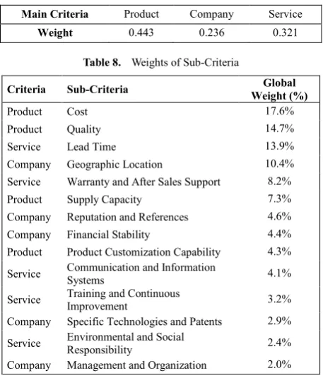
Table 7. Weights of Main Criteria
Main Criteria Product Company Service
Weight 0.443 0.236 0.321
Table 8. Weights of Sub-Criteria
Criteria Sub-Criteria Weight (%) Global
Product Cost 17.6%
Product Quality 14.7%
Service Lead Time 13.9%
Company Geographic Location 10.4% Service Warranty and After Sales Support 8.2%
Product Supply Capacity 7.3%
Company Reputation and References 4.6% Company Financial Stability 4.4% Product Product Customization Capability 4.3% Service Communication and Information Systems 4.1%
Service Training and Continuous Improvement 3.2% Company Specific Technologies and Patents 2.9% Service Environmental and Social Responsibility 2.4% Company Management and Organization 2.0%
Finally, by using equation (4) and equation (5), weights of main criteria and sub-criteria are calculated and given in Table 7 and Table 8 respectively. Global weights of sub-criteria are obtained by multiplying the local weight with corresponding main criterion weight. For example, local weight of cost criterion is obtained as 0.397. It is a sub-criterion of product criterion and the weight of product criterion is 0.443. Therefore, the global weight of cost
criterion can be obtained as 0.176. Global weights of other criteria are determined by the same way.
3.2. Determining the Best Supplier
After determining the criteria weights, we are ready to pass to second step of supplier selection phase, which is evaluating the suppliers and choosing the best one. There are four potential suppliers for the company to work with. Let these suppliers be Supplier A, Supplier B, Supplier C and Supplier D. In order to evaluate them, we apply a survey to high-level managers and buyers of the company. We want from them to evaluate the suppliers according to all criteria. As an example, a manager evaluated the suppliers according to cost criterion in Table 9 and according to quality criterion in Table 10.
Table 9. Evaluation of Suppliers according to Cost Criterion
A B C D
A E FS SW SS
B FW E SW FW
C SS SS E SS
D SW FS SW E
Table 10. Evaluation of Suppliers according to Quality Criterion
A B C D
A E SW SS SW
B SS E FS SS
C SW FW E SW
D SS SW SS E
[image:5.595.308.535.452.507.2]Table 11. Supplier Evaluation Process
Sub-Criteria Weights Sup. A Sup. B Sup. C Sup. D
Cost 0.176 0.30 0.09 0.42 0.19
Quality 0.147 0.15 0.45 0.17 0.23
Lead Time 0.139 0.29 0.51 0.11 0.09
Geographic Location 0.104 0.32 0.27 0.23 0.18
Warranty and After Sales Support 0.082 0.19 0.41 0.23 0.17
Supply Capacity 0.073 0.08 0.32 0.44 0.16
Reputation and References 0.046 0.21 0.17 0.36 0.26
Financial Stability 0.044 0.28 0.21 0.26 0.25
Product Customization Capability 0.043 0.12 0.37 0.35 0.16
Communication and Information Systems 0.041 0.27 0.23 0.29 0.21
Training and Continuous Improvement 0.032 0.17 0.46 0.23 0.14
Specific Technologies and Patents 0.029 0.29 0.18 0.21 0.32
Environmental and Social Responsibility 0.024 0.57 0.12 0.16 0.15
Management and Organization 0.020 0.23 0.24 0.32 0.21
Sum of Weights of Suppliers - 0.240 0.308 0.268 0.184
Sum of Weights of Suppliers (%) - 24% 31% 27% 18%
As a result, it is seen that Supplier B is the best one with a weight of 0.308. According to these results, we can suggest the company to work with Supplier B.
Please note that there is another approach for calculating the weights of alternatives. In that way, the fuzzy weights of criteria and alternatives are put into a fuzzy multiplication process to obtain the fuzzy global weights of alternatives. Then those fuzzy global weights are summed and defuzzification operator is applied in the end. We also try this approach and see that it gives similar results with our approach. We prefer to use a two-step approach for phase I especially in order to show the crisp weights of criteria and crisp weights of suppliers for each criteria.
4. Phase II: Designing the Supply
Chain Network between the
Production Plant and Customers
In this second phase of study, we focus on the design of the supply chain network between production plant, warehouses and customers. More specifically, we try to determine the number and locations of the warehouses, assign the customers to the warehouses and determine the inventory level in each warehouse. We propose a mathematical model in order to make all these decisions. While developing the model, we take care about the company policies mentioned in second section.
Before introducing the mathematical model, it may be beneficial to discuss some issues. Transportation cost plays an important role in total supply chain network cost. It is important to calculate the transportation cost accurately in order to obtain accurate and reliable results from the model. For this reason, we give special attention to this issue. Transportation cost is assumed to be the product of distance and shipping amount in most of the studies in literature. Therefore, if the shipping amount is fixed, it is
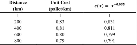
assumed that the transportation cost is a linear function of distance. However, the real life applications do not support this assumption. Unit costs of transportation for different distances are obtained from the company and given below in Table 12.
Table 12. Distance-Based Unit Transportation Costs Distance (km) 1 200 400 600 800 Unit cost (pallet/km) 1.00 0.83 0.81 0.80 0.79
It is seen that the transportation cost does not change linearly as it is assumed. For example, while transporting one unit of product over 200 km costs 166 Turkish Liras (TL), transporting the same product over 400 km costs 324 TL (not 332 TL). Actually, here with the company data we confirm a well-known fact called distance economy. According to distance economy concept, unit transportation cost decreases when the distance increases.
In our example, the company data is provided only for some certain distances. However, the distance between two cities can be any value and we should know the unit transportation costs for all distances. For this reason, we develop a unit transportation cost function by creating a model that minimizes the sum of squares of errors and we obtain the function, 𝑐𝑐(𝑥𝑥) = 𝑥𝑥−0.035 where 𝑐𝑐(𝑥𝑥) is the unit transportation cost and x is the distance. The data obtained from the function is compared with the real company data in Table 13. It is seen that the function,
𝑐𝑐(𝑥𝑥) = 𝑥𝑥−0.035 fits well with the company data and it can
[image:6.595.86.513.91.285.2]be used as a unit transportation cost function.
Table 13. Comparison of the Results of Function and Company Data Distance
(km) (pallet/km) Unit Cost 𝒄𝒄(𝒙𝒙) = 𝒙𝒙−𝟎𝟎.𝟎𝟎𝟏𝟏𝟐𝟐
1 1 1
200 0,83 0,831
400 0,81 0,811
600 0,80 0,799
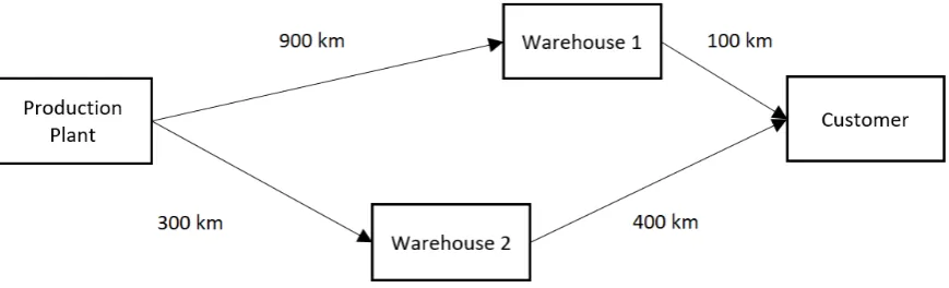
[image:6.595.309.537.672.747.2]Figure 2. A Simple Supply Chain Network
The company has two objectives. First one is minimizing the total supply chain network cost and second one is opening the warehouses as close as possible to customers. Closeness to the customers brings many advantages such as giving fastest possible service, communicating easily and investigating the market conditions easily. Briefly, closeness to the customers increases the service level. For this reason, the second objective can be thought as maximization of service level.
If we want to create a multi-objective model, we must be sure that there is a confliction between objectives. For this reason, we want to clarify whether these two objectives conflict with each other or not. We prove this fact with a simple example given in Figure 2. Suppose that one unit of product will be sent to a customer via the Warehouse 1 or Warehouse 2. When we send the product via Warehouse 1, total transportation cost will be 794.43 TL. On the other hand, if the second warehouse is chosen, the cost will be 570.04 TL. Therefore, if we focus on the cost objective, Warehouse 2 should be chosen. However, if we focus on the closeness objective Warehouse 1 is better than Warehouse 2 since 100 is less than 400. This simple example shows that these two objectives conflict with each other.
4.1. Model
In this subsection, we introduce a multi-objective mathematical model for the second phase of supply chain network design problem. We use weighted sum scalarization method and goal programming approach for this problem. We write two objectives as two goals and try to minimize the total positive deviations from the goals. The reader may notice that the following model is a compact version of the model that was introduced previously by Alegoz and Ozturk [27]. We make some minor changes on the constraints and decision variables to reduce the number of constraints and decision variables. Sets
𝑖𝑖: Set of potential location of warehouses (𝑖𝑖 = 1, …, 81)
𝑗𝑗: Set of customers (𝑗𝑗= 1,…, 81)
Parameters
𝑚𝑚𝑖𝑖: Distances between the production plant and warehouse opened in 𝑖𝑖𝑡𝑡ℎ city.
𝑛𝑛𝑖𝑖𝑖𝑖: Distance between the warehouse opened in 𝑖𝑖𝑡𝑡ℎ city and the customer in 𝑗𝑗𝑡𝑡ℎ city.
𝑑𝑑𝑖𝑖: Average monthly demand of customer in 𝑗𝑗𝑡𝑡ℎ city.
𝑐𝑐𝑖𝑖: Monthly renting and operating cost of warehouse opened in 𝑖𝑖𝑡𝑡ℎ city.
𝑘𝑘: Capacity of warehouses
𝑡𝑡1,𝑡𝑡2: Goal values
𝑤𝑤1,𝑤𝑤2: Weights of goal 1 and goal 2. Decision Variables
𝑥𝑥𝑖𝑖: Amount of product shipped from the production plant to the warehouse opened in 𝑖𝑖𝑡𝑡ℎcity.
𝑠𝑠𝑖𝑖𝑖𝑖: Amount of product shipped from the warehouse opened in 𝑖𝑖𝑡𝑡ℎ city to the customer in 𝑗𝑗𝑡𝑡ℎ city.
𝑦𝑦𝑖𝑖: Binary variable, 1 if a warehouse is opened in 𝑖𝑖𝑡𝑡ℎ city and 0 otherwise
𝑔𝑔1−, 𝑔𝑔1+, 𝑔𝑔2−, 𝑔𝑔2+: Positive and negative deviations from the goal 1 and goal 2.
In this context, the model can be presented as follows.
min𝑧𝑧= 𝑤𝑤1𝑔𝑔1++𝑤𝑤2𝑔𝑔2+ (8)
subject to ∑81𝑖𝑖=1𝑚𝑚𝑖𝑖0.965𝑥𝑥𝑖𝑖+∑𝑖𝑖=181 ∑𝑖𝑖=181 𝑛𝑛0.965𝑖𝑖𝑖𝑖 𝑠𝑠𝑖𝑖𝑖𝑖+∑81𝑖𝑖=1𝑦𝑦𝑖𝑖𝑐𝑐𝑖𝑖+𝑔𝑔1−− 𝑔𝑔1+=𝑡𝑡1 (9)
∑81𝑖𝑖=1∑81𝑖𝑖=1𝑛𝑛𝑖𝑖𝑖𝑖𝑠𝑠𝑖𝑖𝑖𝑖+𝑔𝑔2−− 𝑔𝑔2+=𝑡𝑡2 (10)
𝑥𝑥𝑖𝑖≤k𝑦𝑦𝑖𝑖 ∀𝑖𝑖 (11)
∑81𝑖𝑖=1𝑠𝑠𝑖𝑖𝑖𝑖 ≥ 𝑑𝑑𝑖𝑖 ∀𝑗𝑗 (12)
𝑥𝑥𝑖𝑖≥ ∑81𝑖𝑖=1𝑠𝑠𝑖𝑖𝑖𝑖 ∀𝑖𝑖 (13)
∑81𝑖𝑖=1𝑦𝑦𝑖𝑖≤3 (14)
𝑠𝑠𝑖𝑖𝑖𝑖,𝑥𝑥𝑖𝑖,𝑔𝑔1−,𝑔𝑔1+,𝑔𝑔2−,𝑔𝑔2+ ≥0 and integer, 𝑦𝑦𝑖𝑖∈{0,1} (15)
First of all, observe that the unit transportation cost function is 𝑐𝑐(𝑥𝑥) =𝑥𝑥−0.035 . Therefore, we write the transportation cost between the warehouse opened in 𝑖𝑖𝑡𝑡ℎ city and the customer in 𝑗𝑗𝑡𝑡ℎ city as (𝑛𝑛
𝑖𝑖𝑖𝑖 −0.035.𝑛𝑛
[image:7.595.81.516.82.214.2](𝑛𝑛𝑖𝑖𝑖𝑖−0.035.𝑛𝑛𝑖𝑖𝑖𝑖) is equal to (𝑛𝑛𝑖𝑖𝑖𝑖0.965). Therefore, we can write the transportation cost as (𝑛𝑛𝑖𝑖𝑖𝑖0.965𝑠𝑠𝑖𝑖𝑖𝑖). By the same way, the transportation cost between the production plant and the warehouse opened in 𝑖𝑖𝑡𝑡ℎ city can be written as (𝑚𝑚
𝑖𝑖 0.965.𝑥𝑥
𝑖𝑖). In the model, equation (8) is the objective function, which tries to minimize the total positive deviations from two goals. Here, w values are the weights of the goals. The cost goal is given in equation (9). The first part of that equation is the cost of transportation from the production plant to the warehouses, second part is the cost of transportation from the warehouses to the customers and the third part is fixed cost of renting and operating opened warehouses. Second goal is given in equation (10), which is the closeness goal. It can be observed that 𝑛𝑛𝑖𝑖𝑖𝑖𝑠𝑠𝑖𝑖𝑖𝑖 value is low if the distance between the warehouse and customer is low and high if that distance is high. Equation (11) ensures that it is necessary to open a warehouse in 𝑖𝑖𝑡𝑡ℎ city to make a transportation from the production plant to the warehouse in 𝑖𝑖𝑡𝑡ℎ city. If the warehouse is not opened then there will be no transportation, if it is then there will be at most k units of transportation, where k is the capacity of warehouses. Equation (12) guarantees that demand of each city will be satisfied. Equation (13) is the flow constraint for
warehouses. As a company policy, we limit the maximum number of warehouses with equation (14). Finally, equation (15) sets the sign and type of decision variables.
4.2. Computational Results
The problem is solved by using GAMS optimization software and Baron Solver. When the model is solved only according to cost goal the z value is obtained as 4428661. Therefore, 𝑡𝑡1 value is set as 4428661. By the same way,
𝑡𝑡2 value is set as 2750558. Warehouse capacity is set as total demand, so that it becomes possible to open at least one at most three warehouses. The model decides the exact number of it. The goals are equally weighted since the company managers give equal importance to cost and closeness goals.
Computational results are given below in Table 14. It is seen that 𝑔𝑔1+ value is 177936. This is actually the cost that must be accepted by the company in order to be closer to the customers and in order to increase the service level. Similarly, 𝑔𝑔2+ value is found as 691079 and this must be accepted by the company in order to have less supply chain network cost.
Table 14. Computational Results
Computation
Time (second) 𝒛𝒛 value 𝒈𝒈𝟏𝟏+ value 𝒈𝒈𝟏𝟏+ value Opened Warehouses Monthly Flows (pallet)
583,91 434507.5 177936 691079 Adana, Bilecik, Samsun 1490, 9460, 1517
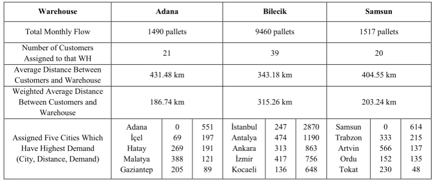
The warehouses are opened in Adana, Bilecik and Samsun. Information about warehouses are given below in Table 15. It is seen that the model opened three warehouses, which is the maximum number of warehouses allowed. This is mainly the result of closeness goal since opening more warehouses allows the company to be closer to customers.
Table 15. Information about Opened Warehouses
Warehouse Adana Bilecik Samsun
Total Monthly Flow 1490 pallets 9460 pallets 1517 pallets
Number of Customers
Assigned to that WH 21 39 20
Average Distance Between
Customers and Warehouse 431.48 km 343.18 km 404.55 km
Weighted Average Distance Between Customers and
Warehouse 186.74 km 315.26 km 203.24 km
Assigned Five Cities Which Have Highest Demand (City, Distance, Demand)
Adana
İçel
Hatay Malatya Gaziantep
0 69 269 388 205
551 197 191 121 89
İstanbul
Antalya Ankara
İzmir
Kocaeli 247 474 313 417 136
2870 1190 863 756 648
Samsun Trabzon Artvin
Ordu Tokat
0 333 566 152 230
614 215 137 135 48
The first warehouse is opened in Adana. Adana is a major city in southern Turkey. 21 cities are assigned to Adana warehouse. When we look at the customers of this warehouse, it is seen that the highest demand is the demand of Adana with 551 pallets/month and the warehouse is located in this city. The second and third highest demands are the demands of
İçel and Hatay with 197 pallets/month and 191 pallets/month respectively. Average distance to its customers is 431.48 km.
[image:8.595.81.511.496.676.2]Bilecik warehouse is determined as the second warehouse. Bilecik is a city located in west of Turkey. Total monthly flow from this warehouse is 9460 pallets, which is more than 2/3 of the company’s monthly flow. In fact, Bilecik is a small city with a demand of only 45 pallets/month. However, opening a warehouse in Bilecik is still logical. Because, firstly the company is located in Bilecik. Secondly, Bilecik is located in the middle of many
major cities such as İstanbul, Ankara, İzmir and Antalya.
Therefore, it is possible to satisfy many major cities’ demands quickly by opening a warehouse in Bilecik. It is seen in Table 15 that average distance from Bilecik warehouse to the customers is 343.18 km and demand-based weighted average distance is 315.26 km.
The third warehouse is opened in Samsun, which is a big city on the north coast of Turkey. Average distance from Samsun warehouse to its customers is 404.55 km. However, demand-based weighted average distance is found as 203.24 km. This shows that Samsun warehouse is located near the cities, which have high demands just like Adana warehouse.
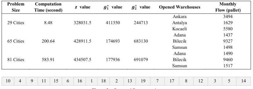
4.3. Necessity of Metaheuristic Approach for Phase II Supply chain network design problem is known as an NP-Hard class problem. For this reason, it becomes difficult or sometimes impossible to solve large size instances by using exact methods as we did in our problem. In such a case, metaheuristic approaches are commonly used. We create three sample problems from our company data in order to show the change of computation time. These problems include 29, 65 and 81 cities respectively. We solve all these problems by using GAMS optimization software and summarized the results in Table 16.
Please note that all these computations are done with a computer that has Intel i5 Processor, 6 GB of RAM and Windows 8.1 Pro Operating System.
It is seen in the Table 16 that the computation time increases prominently when the problem size increases. For instance, when the problem size increases 2.24 times from 29 to 65, computation time increases 47.39 times from 8.48 seconds to 200.64 seconds. From these facts, it is seen that it will be difficult or impossible to solve this
problem with exact methods after some problem size. From another perspective, in some cases the supply chain network may include hundreds or even thousands of cities. In those cases, use of metaheuristic approaches is essential. For this reason, we develop a tabu search based approach, which gives high quality solutions within a reasonable time.
4.4. Proposed Metaheuristic Approach
Representation is crucial for high quality solutions. We propose a permutation representation for the problem discussed in the second phase. If the company has k
customers, the representation includes k cells. In other words, the number of cells are equal to the number of customers. The city numbers are written in each cell as a permutation. If the company wants to open n warehouses (𝑛𝑛 ≤ 𝑘𝑘), then the cities, which are in first n cells are determined as warehouses and all k customers are assigned to those warehouses according to a rule. A sample representation is given in Figure 3. That representation represents a supply chain network that includes 19 customers. The cities are randomly placed in the cells.
According to the representation given in Figure 3 and our proposed approach, if the company wants to open one warehouse, then it will be opened in City 10, which is in first cell and all 19 customers are assigned to that warehouse. Similarly, if the company wants to open two warehouses, they will be opened in cities 10 and 4, which are in first two cells, and all other customers are assigned to these two warehouses according to a rule. By this way, if the company wants to open n warehouses (𝑛𝑛 ≤19), then the first n cells are determined as warehouses and all 19 customers are assigned to those warehouses.
According to our proposed metaheuristic approach, the supply chain network design process includes two steps. At first step, the cities of warehouses are determined and at second step, the customers are assigned to the warehouses. Both two steps are important to obtain high quality results since even if the algorithm finds the right warehouses, different assignments of customers give much different results compared to exact solution. For this reason, it is necessary to focus on both two steps.
Table 16. Computational Results of Three Sample Problems Problem
Size Time (second) Computation 𝒛𝒛 value 𝒈𝒈𝟏𝟏+ value 𝒈𝒈𝟏𝟏+ value Opened Warehouses Flow (pallet) Monthly
29 Cities 8.48 328031.5 411350 244713 Antalya Ankara Kocaeli
3494 1629 5580
65 Cities 200.64 428911.5 174693 683130 Bilecik Adana Samsun
1437 9327 1498
81 Cities 583.91 434507.5 177936 691079 Bilecik Adana Samsun
1490 9460 1517
10 4 9 11 15 6 16 1 18 2 13 19 7 17 8 12 3 5 14
[image:9.595.82.514.594.747.2]We use Glover’s Tabu Search Algorithm in order to determine which warehouses will be opened. In each iteration, the tabu search algorithm will change the warehouse or one of the warehouses and try to jump to a better solution. Since tabu search allows accepting bad solutions, if needed it will jump from the local optimum to any bad solution in order to look for the global optimum. This is one of the most important aspects of tabu search. Secondly, tabu search algorithm has short and long-term memories to keep some information such as previous movements and best solutions. This information makes the algorithm find high quality solutions.
As an example, recall the representation in Figure 3. Suppose that the company wants to open only one warehouse. In this case, it seems that the warehouse will be opened in City 10. In next iteration, tabu search algorithm will change the city of warehouse. It will try all other 18 cities and choose the best one as the new location of warehouse. As an example, suppose that City 6 makes the best improvement in objective function. Then, the tabu search algorithm will swap the cells of City 10 and City 6 and since the first cell is the city of warehouse, the new warehouse will be city 6 as it is seen in Figure 4.
[image:10.595.85.511.532.734.2]The same logic works when the company wants to open two or more warehouses. Again, recall our representation in Figure 3 and suppose that the company wants to open two warehouses. In the beginning, these warehouses are seen as City 10 and City 4. When the tabu search algorithm works, it will try all possible movements, which are 2x17=34 movements, and finds the best movement. Finally, it swaps the places of the two cities. Suppose that the algorithm swapped the places of city 4 and city 16. Then, new two warehouses become cities 10 and 16 as shown in Figure 5.
After this process, the algorithm passes to second step, which is assigning the customers to the warehouses. If the company wants to open one warehouse, of course all the customers will be assigned to that warehouse. However what if the company opens two or more warehouses? How
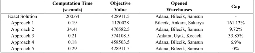
should be the customers assigned to those warehouses? In order to answer these questions we try five different approaches. All these approaches are summarized in Table 17. The gap value in that table refers to the gap between the obtained solution and optimal solution.
In first approach, after determining the warehouses with tabu search algorithm, we assign the customers to the warehouses randomly. It is seen in Table 17 that although the computation time is acceptable compared to exact solution, this approach does not give a high quality solution. It gives a 161.13% gap and this cannot be accepted. In fact, this high gap shows that the assignment should not be done randomly, it should be done according to a rule.
In second approach, after determining the warehouses with tabu search algorithm, we improve this solution with local search approach. For example, the tabu search algorithm finds the warehouses as Adana, Bilecik and Samsun. Then local search begins to work and improves the solution by changing the assignment. Please note that, local search does not change the warehouses, it only works to obtain a better assignment. By using local search instead of random assignment, solution quality is increased and the gap decreased from 161.13% to 9.72%. This is a great improvement. However, this algorithm is not good enough for two reasons. First, since the local search algorithm works in each iteration of tabu search, the computation time increased and this can be a problem especially in very large instances. Secondly, although a gap of 9.72% is much better compared to a gap of 161.13%, it is still not enough to be accepted. Additionally, following inferences can also be made according to these results. Observe that this hybrid algorithm finds the same warehouses compared to optimal solution and the gap is totally a result of wrong assignment. This fact also shows the importance of assignment. Last but not least, it shows that hybrid metaheuristic approaches increase the solution quality but as a disadvantage they also increase the computation time. For this reason, it is important to focus on both solution quality and computation time when using a hybrid approach.
6 4 9 11 15 10 16 1 18 2 13 19 7 17 8 12 3 5 14
Figure 4. Swapping the Places of Cities with Tabu Search – Case I
10 16 9 11 15 6 4 1 18 2 13 19 7 17 8 12 3 5 14
Figure 5. Swapping the Places of Cities with Tabu Search – Case II
Table 17. Various Assignment Approaches Computation Time
(seconds) Objective Value Warehouses Opened Gap
Exact Solution 200.64 428911.5 Adana, Bilecik, Samsun -
Approach 1 0.19 1120028 Bilecik, Ankara, Sakarya 161.13%
Approach 2 34.41 470582.5 Adana, Bilecik, Samsun 9.72%
Approach 3 0.21 574108.5 Ankara, Uşak, Kocaeli 33.85%
Approach 4 0.18 458503.5 Adana, Bilecik, Samsun 6.9%
[image:10.595.86.514.545.619.2] [image:10.595.91.506.642.729.2]In third approach, after determining the warehouses with tabu search, the customers are assigned to the warehouses according to total transportation cost, which is the sum of transportation costs from the production plant to the warehouses and from the warehouses to the customers. Computation time is decreased with this approach. However, it gives a gap of 33.85% and this gap is unacceptable.
In fourth approach, after determining the warehouses with tabu search, the customers are assigned to closest warehouse. This assignment is one of the well-known and commonly used assignments. Both the computation time and gap are decreased with this approach, observe that this is the best approach so far in terms of computation time and gap. The gap is 6.9% and the computation time is only 0.18 seconds. This approach may or may not be accepted but we think that a gap of 6.9% can still be improved. In fact, the gap of 6.9% is again a result of worse assignment since opened warehouses are the same with optimal solution.
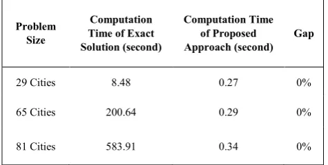
Finally, in fifth approach, after determining the warehouses with tabu search, the customers are assigned to the warehouses according to the objective function. For example, suppose that the tabu search algorithm determined the warehouses as Adana, Bilecik and Samsun and we want to assign Istanbul to any of them. In this case, three objective values are calculated for Istanbul for three assignment cases and the lowest one is determined. Suppose that it is Bilecik. Then, Istanbul is assigned to Bilecik warehouse. By this way, the gap is totally removed and optimal solution is obtained. It means that the solution quality is acceptable. The computation time is also acceptable since it is only 0.29 seconds. This approach is also tested in other test problems we create and the results are summarized in Table 18. It is seen that this approach finds the optimal solution of each problem within a very short time.
Table 18. Comparison of Exact Solution and Proposed Approach
Problem Size
Computation Time of Exact Solution (second)
Computation Time of Proposed
Approach (second) Gap
29 Cities 8.48 0.27 0%
65 Cities 200.64 0.29 0%
81 Cities 583.91 0.34 0%
4.5. Additional Discussions about Computation Time Since metaheuristic approaches are developed especially large size instances of NP-Hard problems, computation time is one of the most important performance indicator for these approaches. For this reason, it is necessary to take care about computation time together with the solution quality. In this subsection, we make additional discussions about computation time of fifth approach.
Suppose that there are 29 cities and the company wants to open exactly two warehouses. In this case, tabu search algorithm tries 54 movements, calculates the objective function for each one, determines the best one and makes that movement. Then, in each iteration, fifth approach calculates two different objective function values for 27 customers and makes the assignment according to those values. Briefly, fifth approach calculates 54 objective function values just like the tabu search. From another perspective, local search algorithm calculates the objective functions of all the swaps of customers with each other, which are 702 swaps. Since swapping the places of x and
y is the same with swapping the places of y and x, this value can be divided by 2 and obtained as 351. Briefly, the assignment algorithm checks the objective function value 351 times when we use local search but only 54 times when we use fifth approach. This difference increases when the problem size increases. For example, for the problem, which has 81 cities (if we want to open exactly 2 warehouses) local search checks the objective value 3081 times but our proposed approach checks the objective value only 158 times. More generally, if there are k cities and the company wants to open exactly 𝑛𝑛 warehouses (𝑛𝑛 ≤ 𝑘𝑘) the local search algorithm makes (𝑘𝑘−𝑛𝑛)(2𝑘𝑘−𝑛𝑛−1) movements and calculates the objective value for each one. For the same problem, fifth approach calculates 𝑛𝑛(𝑘𝑘 − 𝑛𝑛)
objective values. This is the reason of high computation time we see when we use local search and the reason of low computation time when we use fifth approach.
4.6. Additional Discussions about Warehouse Capacity As mentioned earlier, in our problem warehouse capacities are determined according to total demand. So that, it becomes possible to open only one warehouse if it is the best option. In fact, if we limit the warehouse capacity, we actually reduce the possibility of finding better solutions. For example, suppose that total demand is 8000 pallets in a year and the company wants to open at most three warehouses. If we determine the warehouse capacity as 8000 pallets, the model can open at least one and at most three warehouses. However, if we determine the capacity as 3000, the model will open exactly three warehouses but opening two or one warehouse may be better in terms of cost and service level.
[image:11.595.56.294.518.638.2]5. Main Findings
Our analysis shows that MCDM methods are effective tools for addressing the supplier selection problems. By using them, we evaluate the suppliers according to various conflicting quantitative and qualitative criteria simultaneously. Moreover, we see that the supply chain network design problem is an NP-Hard class problem and as the problem size increases, the solution time increases prominently. In order to get over this problem, it is necessary to develop a metaheuristic approach. By this context, we present a representation and develop various hybrid metaheuristic approaches based on tabu search. Some of our approaches give bad results in terms of solution quality or solution time but one of them works well under all problem sizes. In addition to presenting the obtained results from metaheuristics, we also present various insights regarding the gap to optimal solution and computation time.
6. Conclusions and Future Work
Suggestions
In this study, we propose a two-phase supply chain network design approach for a household goods company. We divide the whole problem into two problems since the location of production plant is fixed. We use Buckley’s fuzzy AHP algorithm for the first phase and goal programming for the second phase. In general, it is difficult or sometimes impossible to solve large size instances of this problem with exact algorithms and in such cases, metaheuristic approaches are preferred to obtain solutions. Therefore, we also develop a metaheuristic approach for the problem in second phase. We create three test problems (small, medium, large) to see the performances of proposed metaheuristic approaches in different problem sizes. We solve all of them with exact approaches to make a comparison in terms of both gap and computation time. After comparison, we see that one of our metaheuristic approaches performs well in all three problems.
When we compare the obtained results with company’s recent policy, we see that our proposed approach is better than their recent policy in terms of cost and service level. We cannot give detailed information about the company’s recent policy due to the privacy agreement but we can briefly say that currently the company has only one warehouse in a city located in the middle of Turkey and they make all the transportations from that warehouse. Our approach shows that they can reduce their cost and increase the service level by opening two more warehouses. Moreover, currently, the company works with “Supplier C” which provides the cheapest product but our analysis shows that supplier B is better for them to work with.
In the future, this study can be extended in various ways. Firstly, more complex supply chain structures such as
suppliers, manufacturers, distribution centers, retailers and customers can be studied and efficient representations and metaheuristic approaches for them can be investigated. Secondly, various uncertainties such as supply uncertainty, demand uncertainty and quality uncertainty can be put into account. Thirdly, environmental or social objectives can be used in the model together with these objectives. Finally, different supplier evaluation techniques related to business or engineering perspective of supply chain management can be used and supplier evaluation criteria can be increased with many other criteria.
Acknowledgements
This study is supported by Anadolu University Scientific Research Projects Committee (AUBAP-1501F024).
REFERENCES
[1] Sha, D. Y., & Che, Z. H. (2006). Supply chain network design: partner selection and production/distribution planning using a systematic model. Journal of the operational research society, 57(1), 52-62.
[2] Sabri, E. H., & Beamon, B. M. (2000). A multi-objective approach to simultaneous strategic and operational planning in supply chain design. Omega, 28(5), 581-598.
[3] Guillén, G., Mele, F. D., Bagajewicz, M. J., Espuna, A., & Puigjaner, L. (2005). Multiobjective supply chain design under uncertainty. Chemical Engineering Science, 60(6), 1535-1553.
[4] Meixell, M., & Gargeya, B. (2005). Global supply chain design: A literature review and critique. Transportation Research Part E, 41, 531–550.
[5] Xia, W., & Wu, Z. (2007). Supplier selection with multiple criteria in volume discount environments. Omega, 35, 494– 504.
[6] Zouggari, A., & Benyoucef, L. (2012). Simulation based fuzzy TOPSIS approach for group multi-criteria supplier selection problem. Engineering Applications of Artificial Intelligence, 25, 507–519.
[7] Ávila, P., Mota, A., Pires, A., Bastos, J., & Teixeira, J. (2012) Supplier’s selection model based on an empirical study. Procedia Technology, 5, 625–634.
[8] Rajesh, G., & Malliga, P. (2013). Supplier selection based on AHP QFD methodology. Procedia Engineering, 64, 1283– 1292.
[9] Cárdenas-Barrón, L.E., Gónzalez-Velarde, J.L., &
Treviño-Garza, G., (2015). A new approach to solve the multi-product multi-period inventory lot sizing with supplier selection problem, Computers and Operations Research, 64, 225–232.
multi-objective global supplier selection model under currency fluctuation and price discount. J Ind Eng Int, 13, 161–169.
[11]Wang, F., Lai, X., & Shi, N. (2011). A multi-objective optimization for green supply chain network design. Decision Support Systems, 51, 262–269.
[12]Pazhani, S., Ramkumar, N., Narendran, T., & Ganesh, K. (2013). A bi-objective network design model for multi-period, multi-product closed-loop supply chain. Journal of Industrial and Production Engineering, 30, 264– 280.
[13]Hiremath, N.C., Sahu, S., & Tiwari, M. (2013). Multi objective outbound logistics network design for a manufacturing supply chain. J Intell Manuf, 24, 1071–1084. [14]Cárdenas-Barrón, L.E., & Treviño-Garza, G., (2014). An
optimal solution to a three echelon supply chain network with multi-product and multi-period, Applied Mathematical Modelling, 38 (5-6), 1911–1918.
[15]Yao, M., & Hsu, H. (2009). A new spanning tree-based genetic algorithm for the design of multi-stage supply chain networks with nonlinear transportation costs. Optim Eng, 10, 219–237.
[16]Easwaran, G., & Üster, H. (2009). Tabu search and benders decomposition approaches for a capacitated closed-loop supply chain network design problem. Transportation Science, 43, 301–320.
[17]Costa, A., Celano, G., Fichera, S., & Trovato, E. (2010). A new efficient encoding/decoding procedure for the design of a supply chain network with genetic algorithms. Computers & Industrial Engineering, 59, 986–999.
[18]Cárdenas-Barrón, L.E., Teng, J.T., Treviño-Garza, G., Wee, H.M., & Lou, K.R., (2012). An improved algorithm and solution on an integrated production-inventory model in a three-layer supply chain, International Journal of Production
Economics, 136(2), 384–388.
[19]Castillo-Villar, K., & Herbert-Acero, J. (2014). A metaheuristic-based approach for the capacitated supply chain network design problem including imperfect quality and rework. IEEE Computational Intelligence Magazine, 9, 31–45.
[20]Bruno, G., Esposito, E., Genovese, A., & Passaro, R. (2012) AHP-based approaches for supplier evaluation: problems and perspectives. Journal of Purchasing and Supply Management, 18, 159–172.
[21]Rezaei, J., & Ortt, R. (2013). Multi-criteria supplier segmentation using a fuzzy preference relations based AHP. European Journal of Operational Research, 225, 75–84. [22]Masi, D., Micheli, G., & Cagno, E. (2013). A meta-model
for choosing a supplier selection technique within an EPC company. Journal of Purchasing & Supply Management, 19, 5–15.
[23]Chen, S., & Lee, L. (2010). Fuzzy multiple attributes group decision-making based on the interval type-2 TOPSIS method. Expert Systems with Applications, 37, 2790–2798. [24]Buckley J. (1985) Fuzzy hierarchical analysis. Fuzzy Sets
and Systems, 17, 233–247.
[25]Alegoz, M., & Ozturk Z.K. (2015). A multi objective multi echelon supply chain network model for a household goods company In Hoai An Le Thi et al. (Ed.), Advances in Intelligent Systems and Computing, 359, 307–318.
[26]Saaty, T. (1990). How to make a decision: The analytic hierarchy process. European Journal of Operational Research, 48, 9–26.