Higher Order Splitting Method for Elastic Wave Propagation

Volume 2008, Article ID 291968,31pages doi:10.1155/2008/291968

Research Article

Higher-Order Splitting Method for

Elastic Wave Propagation

J ¨urgen Geiser

Institut f ¨ur Mathematik, Humboldt Universit¨at zu Berlin, Unter den Linden 6, 10099 Berlin, Germany

Correspondence should be addressed to J ¨urgen Geiser,[email protected]

Received 30 July 2008; Accepted 10 November 2008 Recommended by Thomas Witelski

Motivated by seismological problems, we have studied a fourth-order split scheme for the elastic wave equation. We split in the spatial directions and obtain locally one-dimensional systems to be solved. We have analyzed the new scheme and obtained results showing consistency and stability. We have used the split scheme to solve problems in two and three dimensions. We have also looked at the influence of singular forcing terms on the convergence properties of the scheme.

Copyrightq2008 J ¨urgen Geiser. This is an open access article distributed under the Creative Commons Attribution License, which permits unrestricted use, distribution, and reproduction in any medium, provided the original work is properly cited.

1. Introduction

We are motivated by seismological problems that can be studied with higher-order splitting methods scheme. Because of the decomposition, we can save memory and computational time, which is important to study realistic elastic wave propagation. The ideas behind are to split in the spatial directions and obtain locally one-dimensional systems to be solved. Traditionally, using the classical operator splitting methods, we decouple the differential equation into more basic equations. These methods are often not sufficiently stable while also neglecting the physical correlations between the operators. Inspired by the work for the scalar wave equation presented in1, we devise a fourth-order split scheme for the elastic wave equation. From there on, we are going to develop new efficient methods based on a stable variant by coupling new operators and deriving new strong directions. We are going to examine the stability and consistency analyses for these methods and adopt them to linear acoustic wave equationsseismic waves. Numerical experiments can validate our theoretical results and show the possibility to apply our methods.

Section 5with respect to scalar and vectorial problems. Finally, inSection 6, we foresee our future works in the area of splitting and decomposition methods.

2. Mathematical model

The mathematical models are studied in the following subsection. We introduce a scalar and also a vectorial model to distinguish the splitting methods.

2.1. Scalar wave equation

The motivation for the study presented below is coming from a computational simulation of earthquakes, see2, and the examination of seismic waves, see3,4.

We concentrate on the scalar wave equation, see 1, for which the mathematical equations are given by

∂ttuD∇·∇u, inΩ,

ux,0 u0x, utx,0 u1x, inΩ.

2.1

The unknown functionuux, tis considered to be inΩ×0, T⊂Rd×R,where the spatial dimension is given byd.

For three dimensions, we define the diffusion tensor as

D

⎛ ⎜ ⎝

D1 0 0

0 D2 0

0 0 D3

⎞ ⎟

⎠∈R3,_×R3,_{, 2.2}

which describes the wave propagation. Further, the diffusion tensor D is given anisotropic, withD1, D2, D3∈RforD1, D2 ≥D3. The functionsu0xandu1xare the initial conditions

for the wave equation.

We deal with the following boundary conditions:

ux, t u3, Dirichlet boundary condition,

∂ux, t

∂n 0, Neumann boundary condition,

D∇ux, t uout, Outflow boundary condition,

2.3

where all boundary conditions are on∂Ω×T.

2.2. Elastic wave propagation

ρ∂ttUμ∇2U λμ∇∇·U f, 2.4a

Ut0,x g0x, 2.4b

∂tUt0,x g1x, 2.4c

where U ≡ Ux, tis the displacement vector with componentsu, vT or u, v, wT in two and three dimensions, f, g0, and g1are known initial functions, and finally x x, y, zT. This

equation is commonly used to simulate seismic events.

In seismology, it is common to use spatially singular forcing terms which can look like

fFδxgt, 2.5

where F is a constant vector. A numeric method for2.4aneeds to approximate the Dirac function correctly in order to achieve full convergence.

3. Discretization methods

In this section, we discuss the discretization methods, both for time and space, to construct higher order methods. Because of the combination of both discretization, we can further show also higher-order methods for the splitting schemes, see also1.

3.1. Discretization of the scalar equation

At first, we underly finite difference schemes for the time and spatial discretization.

For the classical wave equation, this discretization is the well-known discretization in time and space.

Based on this discretization, the time is discretized as

Utt,i Un1

i −2Uni Uni−1 Δt2 ,

Utn _{ux, t, Utt}n _{utx, t,}

3.1

where the indexirefers to the space pointxiandΔttn1_−tn_{is the time step. We apply finite} difference methods for the spatial discretization. The spatial terms and the initial conditions are given as

Uxx,n U n

i1−2UinUni−1

Δx2 ,

Utn _{ux, t, U} t

tn _{utx, t,}

3.2

Then the two-dimensional equation,

uttD1uxxD2uyy inΩ,

ux, y,0 u0x, y, utx, y,0 u1x, y,

ux, y, t u2 on∂Ω,

3.3

is discretized with the unconditionally stable implicitη-method, see5,

Un1

i,j −2Uni,jUni,j−1 Δt2

D1

Δx2

ηU_in₁1_,j−2U_i,jn1U_in₋₁1_,j 1−2ηUn_i1,j−2U_i,jn U_in_−1,j ηU_in−₁1_,j−2Un_i,j−1Un_i−−₁1_,j

D2

Δy2

ηUn

i,j1−2Uni,jUni,j−1 1−2η

Un

i,j1−2Uni,jUni,j−1 η

Un−1

i,j1−2Ui,jn−1Uni,j−−11

,

3.4

whereΔxandΔyare the grid width inxandyand 0≤η≤1. The initial conditions are given byUx, y, tn _{ux, y, t}n_{andUx, y, t}n−1 _{ux, y, t}n_{−Δtutx, y, t}n_.

These discretization schemes are adopted to the operator splitting schemes.

On the finite differences grid,Δtcorresponds to the time step, andhx,hyare the grid sizes in the different spatial directions. The timenΔtis denoted by tn_{, and i, j refer to the} spatial coordinates of the grid pointihx, jhy. Let un denote the grid function on the time leveln, andun_i,j be the specific value of un_{at pointi, j.}

InSection 3.2, we describe the traditional splitting methods for the wave equation.

3.2. Discretization of the vectorial equation

One of the first practical difference scheme with central differences used everywhere was introduced in3. To save space we exemplify it and some newer schemes in two dimensions first.

If we discretize uniformly in space and time on the unit square, we get a grid with grid pointsxj jh,yk kh,tn nΔt, whereh > 0 is the spatial grid size andΔtthe time step. Defining the grid function Un

j,k Uxj, yk, tn, the basic explicit scheme is

ρU n1

j,k −2Unj,kUnj,k−1

Δt2 M2U

n j,kf

n

j,k, 3.5

whereM2is a difference operator

M2

⎛

⎝λ2μDx

2

μDy2

λμDx

0D

y

0

λμDx

0D

y

0 λ2μDy

2

μDx2

⎞

and we use the standard difference operator notation:

Dxvj,k 1 h

vj1,k−vj,k , D₋xvj,k Dxvj−1,k, Dx0

1 2

DxD₋x , Dx2 DxDx₋. 3.7

M2is a second-order difference approximation of the right-hand side operator of2.4a. This

explicit scheme is stable for time steps satisfying6

Δt < h

λ3μ. 3.8

ReplacingM2withM4, a fourth-order difference operator given by

M4 ⎛ ⎜ ⎜ ⎜ ⎜ ⎜ ⎜ ⎜ ⎜ ⎜ ⎜ ⎜ ⎜ ⎜ ⎜ ⎜ ⎜ ⎝

λ2μ

1−h

2

12D x2

Dx2μ

1−h

2

12D y2

Dy2

λμ

1−h

2 6 D x2 Dx 0

1−h

2

6 D y2

D₀y

λμ

1−h

2 6 D x2 Dx 0

1−h

2

6 D y2

D₀y

λ2μ

1−h

2

12D y2

Dy2

μ

1− h

2

12D x2

Dx2

⎞ ⎟ ⎟ ⎟ ⎟ ⎟ ⎟ ⎟ ⎟ ⎟ ⎟ ⎟ ⎟ ⎟ ⎟ ⎟ ⎟ ⎠ , 3.9

and using the modified equation approach to eliminate the lower-order error terms in the time difference6, we obtain the explicit fourth-order scheme

ρU n1

j,k −2Unj,kUnj,k−1

Δt2 M4U

n

j,kfnj,k Δt2

12

M2

2Unj,kM2fni,j∂ttfni,j , 3.10

whereM2

2is a second-order approximation to the squared right-hand side operator in2.4a.

As it only needs to be second-order accurate,M2₂has the same extent in space asM4and no

more grid points are used. This scheme has the same time step restriction as3.8. In1the following implicit scheme for the scalar wave equation was introduced:

ρ

Un1

j,k −2Unj,kUnj,k−1 Δt2 M4

Whenθ 1/12,the error of this scheme is fourth-order in time and space. For thisθvalue, it is, however, only conditionally stable, allowing a time step approximately 45% larger than 3.8 forθ∈0.25,0.5,it is unconditionally stable.

In order to make it competitive with the explicit scheme3.10, we provide an operator split version of the implicit scheme3.11. This is made complicated by the presence of the mixed derivative terms that couple different coordinate directions.

4. Higher-order splitting method for the wave equations

In this section, we discuss the splitting methods for the wave equations. The higher order results as a combination between the spatial and time discretization method and the weighting factors in the splitting schemes.

4.1. Traditional splitting methods for the scalar wave equation

Our classical method is based on the splitting method of5,7.

The classical splitting methods alternating direction methodsADIsare based on the idea of computing the different directions of the given operators. Each direction is computed independently by solving more basic equations. The result combines all the solutions of the elementary equations. So we obtain more efficiency by decoupling the operators.

The classical splitting method for the wave equation starts from

∂ttut ABCut ft, t∈

tn, tn1 ,

utn u0, u

tn u1,

4.1

where the initial functionsu0andu1are given. We could also apply foru1thatutn utn−

utn−1_{/ΔtOΔt u}

1. Consequently, we haveutn−1≈u0−Δtu1. The right-hand sideft

is given as a force term.

The spatial discretization terms are given by

A ∂

2

∂x2, B

∂2

∂y2, C

∂2

∂z2, 4.2

where the approximated discretization is given by

Aux, y, z ≈ ux Δx, y, z−2ux, y, z ux−Δx, y, z

Δx2 ,

Bux, y, z ≈ ux, y Δy, z−2ux, y, z ux, y−Δy, z

Δy2 ,

Cux, y, z ≈ ux, y, z Δz−2ux, y, z ux, y, z−Δz

Δz2 .

We could decouple the equation into 3 simpler equations obtaining a method of second order:

u−2utn utn−1 Δt2Aηu 1−2ηutn ηutn−1

Δt2_Butn _Δt2_Cutn

Δt2_ηftn1 _1−2ηftn _ηftn−1 _,

4.4a

u−2utn utn−1 Δt2Aηu 1−2ηutn ηutn−1

Δt2_{Bηu 1−2ηut}n _ηutn−1

Δt2_Cutn _Δt2_ηftn1 _1−2ηftn _ηftn−1 _,

4.4b

utn1 _−2utn _utn−1 _Δt2_{Aηu 1−2ηut}n _ηutn−1

Δt2_{Bηu 1−2ηut}n _ηutn−1

Δt2_Cηutn1 _1−2ηutn _ηutn−1

Δt2_ηftn1 _1−2ηftn _ηftn−1 _,

4.4c

where the result is given asutn1_{with the initial conditionsut}n _u

0,utn−1 u0−Δtu1,

andη ∈0,0.5. A fully coupled method is given forη 0 and for 0< η ≤1 the decoupled method consists of a composition of explicit and implicit Euler methods.

We have to compute the first equation4.4aand get the resultuthat is a further initial condition for the second equation4.4b; after whose computation we obtainu. In the third equation4.4c, we have to putuas a further initial condition and get the resultutn1.

The underlying idea consists of the approximation of the pairwise operators:

Δt2_Aηu−2utn _utn−1 _≈0,

Δt2_Bηu−2utn _utn−1 _≈0, 4.5

which we can raise to second order.

4.2. Boundary splitting method for the scalar wave equation

The time-dependent boundary conditions also have to be taken into account for the splitting method. Let us consider the three-operator example with the equations

∂ttut ABCut ht, t∈

tn, tn1 ,

whereAD1x, y, z∂2/∂x2,BD2x, y, z∂2/∂y2, andCD3x, y, z∂2/∂z2are the

spatial operators. The wave-propagation functions are as follows:

D1x, y, z, D2x, y, z, D3x, y, z:R3−→R. 4.7

Hence, for 3 operators, we have the following second-order splitting method:

u−2utn utn−1 Δt2Aηu 1−2ηutn ηutn−1

Δt2_Butn _Δt2_Cutn

Δt2_ηhtn1 _1−2ηhtn _ηhtn−1 _,

u−2utn utn−1 Δt2Aηu 1−2ηutn ηutn−1

Δt2_{Bηu 1−2ηut}n _ηutn−1

Δt2_Cutn _Δt2_ηhtn1 _1−2ηhtn _ηhtn−1 _,

utn1 −2utn utn−1 Δt2Aηu 1−2ηutn ηutn−1

Δt2_{Bηu 1−2ηut}n _ηutn−1

Δt2_Cηutn1 _1−2ηutn _ηutn−1

Δt2_ηhtn1 _1−2ηhtn _ηhtn−1 _,

4.8

where the result is given asutn1_.

The boundary values are given by the following.

1Dirichlet values. We have to use the same boundary values for all 3 equations. 2Neumann values. We have to decouple the values into the different directions:

∂u

∂n 0 4.9

is split in

∂u ∂xnx

∂u ∂yny

∂u ∂znz0;

∂u ∂n 0

is split in

∂u ∂xnx

∂u ∂yny

∂u ∂znz0;

∂utn1 ∂n 0

4.11

is split in

∂u ∂xnx

∂u ∂yny

∂un1

∂z nz0. 4.12

3Outflowing values, we have to decouple the values into the different directions:

nD∇uuout 4.13

is split in

D1∂xun xD2∂yun yD3∂zun zuout;

nD∇uuout

4.14

is split in

D1∂xun xD2∂yun yD3∂zun zuout;

nD∇un1_u

out

4.15

is split in

D1∂xunxD2∂yun yD3∂zun1nzuout, 4.16

where n is the outer normal vector and the anisotropic diffusion D, see2.2, is the parameter matrix to the wave-propagations.

We have the following initial conditions for the three equations:

utn u0,

utn−1 u0−Δtu1Δt 2

2

ABCu0f

tn OΔt3 ,

utn−1 u0−Δtu1Δt 2

2

ABC

u0−Δt

3 u1 Δt2

12ABCu0

Δt2 2 f

tn −Δt

3

6 ∂ftn

∂t Δt4

24 ∂2_ftn

∂t2 O

Δt5 _.

Remark 4.1. By solving the two or three splitting steps, it is important to mention that each solutionu, u, and uis corrected only once by using the boundary conditions.

Otherwise, an “overdoing” of the boundary conditions takes place.

4.3. LOD method: locally one-dimensional method for the scalar wave equation

In the following, we introduce the LOD method as an improved splitting method while using prestepping techniques.

The method was discussed in1and is given by

un1,0_−2un_un_{−1 Δt}2_ABun_,

un1,1_−un1,0 _Δt2_ηAun1_−2un_un−1 _,

un1_−un1,1 _Δt2_ηBun1_−2un_un−1 _,

4.18

whereη∈0.0,0.5andA, Bare the spatial discretized operators. If we eliminate the intermediate values in4.18, we obtain

un1−2unun−1 Δt2ABηun1 1−2ηunηun−1 Bηun1−2unun−1 , 4.19

whereBηη2Δt4ABand thusBηun1−2unun−1 OΔt6. So, we obtain a higher-order method.

Remark 4.2. Forη∈0.25,0.5,we have unconditionally stable methods and for higher order we useη1/12. Then, for sufficiently small time steps, we get a conditionally stable splitting method.

4.4. Stability and consistency analysis for the LOD method of the scalar wave equation

The consistency of the fourth-order splitting method is given in the next theorem.

Hence, we assume discretization orders ofOhp_{,p 2,4, for the discretization in} space, wherehhxhyis the spatial grid width.

Then we obtain the following consistency result for our method4.18.

Theorem 4.3. The consistency of the LOD method is given by

utt−Au−

∂ttu−Au O

Δt2 _{, 4.20}

Proof. We add4.18and obtain the following, see also1:

∂ttun−A

θun1 1−2θunθun−1 −Bun1−2unun−1 0, 4.21

whereBθ2_Δt2_A 1A2.

Therefore, we obtain a splitting error ofBu n1_−2un_un−1_.

Sufficient smoothness assumed that we have un1_−2un _un−1 _OΔt2_{, and we}

obtainBu n1_−2un_un−1 _OΔt4_.

Thus, we obtain a fourth-order method if the spatial operators are also discretized as fourth-order terms.

The stability of the fourth-order splitting method is given in the following theorem.

Theorem 4.4. The stability of the method is given by

1−Δt2B 1/2∂_tun2Pun, θ ≤1−Δt2B 1/2∂_tu02Pu0, θ , 4.22

whereθ∈0.25,0.5andP±uj_{, θ:θAu} j_{, u}j _θAu j±1_{, u}j±1 _1−2θAu j_{, u}j±1_.

Proof. We have to proof the theorem for a test function∂tun, where ∂tdenotes the central difference.

Forj≥1,we have

1−Δt2B ∂ttuj, ∂tuj A

θuj1−1−2θujθuj−1 , ∂tuj 0. 4.23

Multiplying withΔtand summarizing overjyield

n

j1

1−Δt2B ∂ttuj, ∂tuj Δt A

θuj1−1−2θujθuj−1 , ∂tuj , ∂tuj Δt0. 4.24

We can derive the identities

1−Δt2_{B ∂ttu}j_{, ∂tu}j _Δt 1

21−Δt

2_B 1/2_∂

tuj

2₋1

21−Δt

2_B 1/2_∂−

tuh

2

,

Aθuj1_−1−2θuj_θuj−1 _{, ∂}

tuj Δt 1 2

P_uj_{, θ − P}−_uj_{, θ ,}

4.25

and obtain the result

_1−Δt2_B 1/2

∂_tun2Pun, θ ≤1−Δt2B 1/2∂_tu02Pu0, θ , 4.26

see also the idea of1.

Remark 4.5. Forθ1/12, we obtain a fourth-order method.

To compute the error of the local splitting, we have to use the multiplierA1A2, thus

Remark 4.6. 1The unconditional stable version of LOD method is given forθ∈0.25,0.5. 2The truncation error isOΔt2_hp_{,p≥2,forθ∈0,0.5.}

3θ1/12,we have a fourth-order method in timeOΔt2_hp_{, p≥2.} 4θ0 we have a second-order explicit scheme.

5For the stable version of the LOD method, the CFL condition should be taken into account for allθ∈0,0.25withCFL Δt2_/Δx2

maxDmax, wherexmaxare the maximal spatial

step andDmaxare the maximal wave-propagation parameter in space.

In the next subsections, we discuss the higher-order splitting methods for the vectorial wave equations.

4.5. Higher-order splitting method for the vectorial wave equation

In the following, we present a fourth-order splitting method based on the basic scheme3.11. We split the operatorM4into three parts:Mxx,Myy, andMxy, where we have

Mxx ⎛ ⎜ ⎜ ⎜ ⎝

λ2μ

1−h

2

12D x2

Dx2 0

0 μ

1−h

2

12D x2

Dx2

⎞ ⎟ ⎟ ⎟ ⎠, Myy ⎛ ⎜ ⎜ ⎝ μ

1−h

2

12D y2

Dy2 0

0 λ2μ

1−h

2

12D y2

Dy2

⎞ ⎟ ⎟

⎠,

Mxy M4− Mxx− Myy.

4.27

Our proposed split method has the following steps:

1 ρU

∗

j,k−2U n j,kU

n−1

j,k

Δt2 M4U

n

j,kθfnj,k1 1−2θfnj,kθfnj,k−1,

2 ρU

∗∗

j,k−U∗j,k

Δt2 θMxx

U∗∗

j,k−2Unj,kUnj,k−1 θ 2Mxy

U∗

j,k−2Unj,kUnj,k−1 ,

3 ρU n1

j,k −U∗∗j,k

Δt2 θMyy

Un1

j,k −2Unj,kUnj,k−1 θ 2Mxy

U∗∗

j,k−2Unj,kUnj,k−1 .

4.28

Here, the first step is explicit, while the second and third steps treat the derivatives along the coordinate axes implicitly and the mixed derivatives explicitly. This is similar to how the mixed case is handled for parabolic problems8.

4.6. Stability and consistency of the higher-order splitting method of the vectorial wave equations

The consistency of the fourth-order splitting method is given in the following theorem. We have for all sufficiently smooth functions Ux, tthe following discretization order:

M4Uμ∇2U λμ∇∇·U O

h4 . 4.29

Furthermore, the split operators are also discretized with the same order of accuracy. Then, we obtain the following consistency result for the split method4.28.

Theorem 4.7. The split method has a splitting error which for smooth solutions U isOΔt4_{, where}

it is assumed thatΔtOh.

Proof. We assume in the following that f 0,0T. We add4.28and obtain, like in the scalar case1, the following result for the discretized equations

DtD₋tUn_j,k− M4

θUn_j,k1 1−2θU_j,kn θUn_j,k−1 − N4,θ

Un1

j,k −2U n j,kU

n−1

j,k 0, 4.30

whereN4,θθ2Δt2MxxMyyMxxMxyMxyMyy θ3Δt4MxxMyyMxy. We, therefore, obtain a splitting error ofN4,θUn_j,k1−2Un_j,kUn_j,k−1.

For sufficient smoothness, we have Un1

j,k −2Unj,k Unj,k−1 OΔt2 and we obtain N4,θUn1−2UnUn−1 OΔt4.

It is important that the influence of the mixed terms can be also be discretized as fourth-order method and, therefore, the terms are canceled in the proof.

For the stability, we have to denote an appropriate norm, which is in our case the L2Ω.

In the following, we introduce the notation of the norms.

Remark 4.8. For our system, we extend theL2-norm as

U2

L2 U,UL2

Ω U

2_{dx, 4.31}

where U2 _u2_v2_{or U}2_u2_v2_w2_{in two and three dimensions.}

Remark 4.9. For a discrete grid function Un

j,k, theL2-norm is given as

Ω

Un jk

2

dx Δx2 M

j,k

U_j,kn , 4.32

whereΔxis the uniform grid length inxandy,Mis the number of grid points inxandy. Further,Un

Remark 4.10. The matrix

N4,θθ2Δt2

MxxMyyMxxMxyMxyMyy θ3Δt4MxxMyyMxy, 4.33

where Mxx, Myy, and Mxy are symmetrical and positive-definite matrices, therefore, the matrixN4,θis also symmetrical and positive-definite.

Furthermore, we can estimate the norms and define a weighted norm, see9,10.

Remark 4.11. The energy norm is given as

N4,θU,U _L2

Ω

N4,θU U dx. 4.34

Consequently, we can denote

_N4,θU≤ωU ∀U∈Hd, 4.35

whereω∈Ris the weight andN4,θis bounded.dis the dimension, andHis Sobolev-space, see11.

The stability of the fourth-order splitting method is given in the following theorem.

Theorem 4.12. Letθ∈0.25,0.5, then the implicit time-stepping algorithm, see3.5, and the split procedure, see4.28, are unconditionally stable. One can estimate the split procedure iteratively as

1−Δt2ω 1/2DtUn_j,k2PUn_j,k, θ ≤1−Δt2ω 1/2DtU0_j,k2PU0_j,k, θ , 4.36

where one hasP±Un

j,k, θ:θM4Unj,k,Unj,kθM4Unj,k±1,Unj,k±11−2θM4Unj,k,Unj,k±1andP± ≥ 0 forθ∈0.25,0.5. Further, 1−Δt2_{ω ∈Ris the factor for the weighted normI−Δt}2_N

4,θU≤ωU for all U∈Hd_.

We have to prove the iterative estimate for the split procedure and the proof is given as follows.

Proof. To obtain an energy estimate for the scheme, we multiply with a test-functionDt

0Unj,k. The following result is given for the discretized equations, see also4.30:

I −Δt2_N

4,θ DtD−tUnj,k− M4

θUn_j,k1 1−2θU_j,kn θUn_j,k−1 0. 4.37

So forn≥1, we can rewrite4.37for the stability proof as follows:

I −Δt2_N

4,θ DtDt−Unj,k, Dt0Unj,k −

M4

Multiplying withΔtand summarizing over the time levels, we obtain

n

I−Δt2_N

4,θ DtDt−Unj,k, D0tUnj,k Δt−

n

M4

θUn_j,k11−2θUn_j,kθU_j,kn−1 , D₀tUn_j,k Δt0, 4.39

for each term of the sum, one can derive the following identities. So forI −Δt2_N

4,θ, we have

I −Δt2_N

4,θ DtDt₋U_j,kn , Dt₀Un_j,k Δt1 2

I −Δt2_N

4,θ Dt−Dt₋ Un_j,k,

DtDt₋ Un_j,k

Ω

I −Δt2_N

4,θ Dt −D−t TDtDt− Unj,kdx

≤1−Δt2ω

Ω

DtUn_j,k 2D₋tUn_j,k 2dx,

4.40

where the operator I −Δt2_N

4,θ is symmetric and positive-definite and we can apply the weighted norm, seeRemark 4.11and11.

We obtain the following result:

1−Δt2ω

Ω

DtUn_j,k 2Dt₋Un_j,k 2dx 1

21−Δt

2_ω 1/2

DtUn_j,k2−1

21−Δt

2_ω 1/2

Dt₋Un_j,k2.

4.41

Further, for−M4, we have

− M4

θUn_j,k1 1−2θUn_j,kθUn_j,k−1 , Dt₀Un_j,k Δt 1 2

P_Un

j,k, θ − P−

Un j,k, θ

. 4.42

Due to the result of the operators:

P−_Un

j,k, θ P

Un−1

j,k , θ , Dt−Unj,k DtUnj,k−1, 4.43

we can recursively derive the following result:

1−Δt2_ω 1/2_Dt

Unj,k

2_PUn

j,k, θ ≤1−Δt2ω

1/2

Dt

U0j,k

2_PU0

j,k, θ , 4.44

Remark 4.13. Forθ1/12, the split method is fourth-order accurate in time and space.

See the following theorem.

Theorem 4.14. One obtains a fourth-order accurate scheme in time and space for the split method, see4.28, whenθ1/12. That reads

DtDt₋Un_j,k− 1 12M4

Un1

j,k −2Unj,kUj,kn−1 M4Unj,kN4,θ

Un1

j,k −2Unj,kUnj,k−1 0, 4.45

whereM4is a fourth-order discretization scheme in space.

The proof is given as follows.

Proof. We consider the following Taylor-expansion:

∂ttUn_j,kDtDt₋Un_j,k−Δt

2

12 ∂ttttU n j,kO

Δt4 _{. 4.46}

Furthermore, we have

∂ttttUnj,k≈ M4∂ttUnj,k, 4.47

and we can rewrite4.46as

∂ttUn_j,k ≈DtDt₋Un_j,k−Δt

2

12M4∂ttU n j,kO

Δt4

≈DtDt₋Un_j,k−Δt

2

12M4

Un1

j,k −2Unj,kUnj,k−1 O

Δt4 _.

4.48

So the fourth-order time-stepping algorithm can be formulated as

DtDt₋Un_j,k− 1 12M4

Un1

j,k −2Unj,kUj,kn−1 − M4Unj,k0. 4.49

The split method4.28becomes

DtDt₋Un_j,k− 1 12M4

Un1

j,k −2Unj,kUnj,k−1 − M4Unj,k− N4,1/12

Un1

j,k −2Unj,kUnj,k−1 0, 4.50

and we obtain a fourth-order split schemecf. the scalar case1.

Remark 4.15. As follows formTheorem 4.14, we obtain a fourth-order in time forθ 1/12. For the stability analysis, the method is conditional stable forθ ∈ 0,0.25. So the splitting method will not restrict our stability condition for the fourth-order method withθ1/12.

5. Numerical experiments

In this section, we present the numerical experiments for scalar and vectorial wave equations. The benefit of the splitting methods is discussed.

5.1. Numerical examples of the scalar wave equation

To test examples for the scalar wave equations, we discussed numerical experiments, which are based on analytical solutions. We present various boundary conditions and also spatial-dependent propagation functions. The benefit of the splitting method to reduce the computational amount is discussed with respect to the approximation errors.

5.1.1. Test example 1: problem with analytical solution and Dirichlet boundary condition

We deal with a two-dimensional example with constant coefficients where we can derive an analytical solution:

∂ttuD12∂xxuD22∂yyu, inΩ×0, T,

ux, y,0 u0x, y sin

1 D1

πx

sin

1 D2

πy

, onΩ,

∂tux, y,0 u1x, y 0, onΩ,

ux, y, t sin

1 D1πx

sin

1 D2πy

cos√2πt , on∂Ω×0, T,

5.1

where the initial conditions can be written as ux, y, tn _u

0x, y and ux, y, tn−1

ux, y, tn1 _{ux, y,Δt.}

The analytical solution is given by

uanax, y, t sin

₁

D1πx

sin

₁

D2πy

cos√2πt . 5.2

For the approximation error, we choose theL1-norm.

TheL1-norm is given by

errL1:

i,j1,...,m Vi,ju

xi, yj, tn −uana

xi, yj, tn , 5.3

where uxi, yj, tn _{is the numerical and u}

anaxi, yj, tn is the analytical solution and Vi,j

ΔxΔy.

Our test examples are organized as follows.

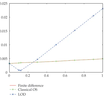
1The non-stiffcase. We chooseD1 D2 1 with a rectangle as our model domain

Ω 0,1×0,1. We discretize withΔx1/16 andΔy1/16 andΔt1/32 and choose our parameterη between 0 ≤ η ≤ 1. The exemplary function values unum

0 0.002 0.004 0.006 0.008 0.01 0.012 0.014 0.016 0.018 0.02

0 0.2 0.4 0.6 0.8 1

Finite difference Classical OS LOD

Figure 1: Numerical error for standard and modified methods, with respect to the η parameter and Dirichlet boundary conditions.

−1 −0.5 0 0.5 1

1 0.5

0 0 0.2 0.4 0.6

0.8 1 Numeric solutionΔx1/32,Δy1/32,

Δt1/64,η0.5

a

−2 0 2 4 6 8 ×10−3

1 0.5

0 0 0.2 0.4 0.6

0.8 1 Analytic-numericΔx1/32,Δy1/32,

Δt1/64,η0.5

b

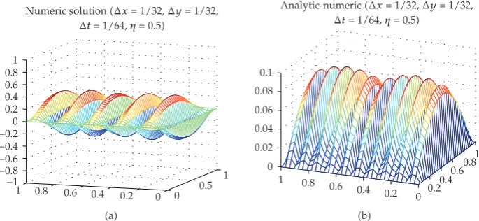
Figure 2: Numerical resolution of the wave equation: numerical approximationaand error functionsb

for the Dirichlet boundary conditionsΔx Δy1/32,Δt1/64,D11,D21 classical method.

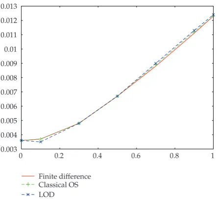
2The stiffcase. We chooseD1 D2 0.01 with a rectangle as our model domain

Ω 0,1×0,1. We discretize withΔx1/32 andΔy1/32 andΔt1/64 and choose our parameterη between 0 ≤ η ≤ 1. The exemplary function values unum

anduanaare taken from the point0.5,0.5625.

The experiments are done with the uncoupled standard discretization methodi.e., the finite differences methods for time and space, and with the operator splitting methods, i.e., the classical operator splitting method and the LOD method.

0.0335 0.034 0.0345 0.035 0.0355 0.036 0.0365 0.037 0.0375 0.038

0 0.2 0.4 0.6 0.8 1

Finite difference Classical OS LOD

Figure 3: Numerical error for standard and modified methods, with respect to theηparameter, Dirichlet boundary conditions and stiffcaseΔx Δy1/32,Δt1/64,D11,D20.01.

−1 −0.8 −0.6 −0.4 −0.2 0 0.2 0.4 0.6 0.8 1

1 0.8 0.6 0.4 0.2 0 0 0.5 1 Numeric solutionΔx1/32,Δy1/32,

Δt1/64,η0.5

a

0 0.02 0.04 0.06 0.08 0.1

1 _0.8

0.6 _0.4

0.2 ₀ 0.2 0.40.6

0.81 Analytic-numericΔx1/32,Δy1/32,

Δt1/64,η0.5

b

Figure 4: Numerical approximation and error function for the Dirichlet boundary in the stiffcaseΔx

Δy1/32,Δt1/64,D11,D20.01.

The numerical errors for the stiff case with Dirichlet boundary conditions are presented inFigure 3and their results inFigure 4.

Remark 5.1. In the experiments, we compare the non-splitting with the splitting methods. We obtain nearly the same results and could see improved results for the LOD method, which is forη1/12 a fourth-order method.

0.003 0.004 0.005 0.006 0.007 0.008 0.009 0.01 0.011 0.012 0.013

0 0.2 0.4 0.6 0.8 1

Finite difference Classical OS LOD

Figure 5: Numerical error for standard and modified methods, with respect to the η parameter and Neumann boundary conditions.

5.1.2. Test example 2: problem with analytical solution and Neumann boundary condition

In this example, we modify our boundary conditions with respect to the Neumann boundary. We deal with our 2D example where we can derive an analytical solution:

∂ttuD2₁∂xxuD2₂∂yyu, inΩ×0, T,

ux, y,0 u0x, y sin

1 D1

πx

sin

1 D2

πy

, onΩ,

∂tux, y,0 u1x, y 0, onΩ,

∂ux, y, t ∂n

∂uanalyx, y, t

∂n 0, on∂Ω×0, T,

5.4

where Ω 0,1×0,1. D1 1, D2 0.5 and the initial conditions can be written as

ux, y, tn _u

0x, yandux, y, tn−1 ux, y, tn1 ux, y,Δt.

The analytical solution is given as

canalyx, y, t sin

1 D1πx

sin

1 D2πy

cos√2πt . 5.5

We have the same discretization methods as in test example 1.

−1 −0.8 −0.6 −0.4 −0.2 0 0.2 0.4 0.6 0.8 0

1 0.8 0.6 0.4 0.2 0 0 0.5 1 Numeric solutionΔx1/32,Δy1/32,

Δt1/64,η0

a

0 0.5 0 1.5 2 2.5 3 3.5 4 ×10−3

1 0.8 0.6 _{0.4 0.2} 00.2

0.04.6 0.81 Analytic-numericΔx1/32,Δy1/32,

Δt1/64,η0

b

Figure 6: Numerical resolution of the wave equation: numerical approximationaand error functionsb

for the Neumann boundary conditionΔx Δy1/32,Δt1/64,D11,D21 classical method.

Remark 5.2. In the experiments, we can obtain the same accuracy as for the Dirichlet boundary conditions. More accurate results are gained by the LOD method with smallη. We obtain also stable results in our computations.

5.1.3. Test example 3: spatial-dependent wave equation

In this experiment, we apply our method to the spatial-dependent problem, given by

∂ttuD1x, y∂xxuD2x, y∂yyu, inΩ×0, T,

ux, y, tn u0, ∂tu

x, y, tn u1, on∂Ω×0, T,

ux, y, t u2, on∂Ω×0, T,

5.6

whereD1x, y 0.1x0.01y0.01,D2x, y 0.01x0.1y0.1.

To compare the numerical results, we cannot use an analytical solution, that is why in a first prestep we are computing a reference solution. The reference solution is done with the finite difference scheme with fine time and space steps.

Concerning the choice of the time steps, it is important to consider the CFL condition, that is now based on the spatial coefficients.

Remark 5.3. We have assumed the following CFL condition:

Δt < 0.5 minΔx,Δy maxx,y∈ΩD1x, y, D2x, y

. 5.7

0 0.005 0.01 0.015 0.02 0.025

0 0.2 0.4 0.6 0.8 1

Finite difference Classical OS LOD

Figure 7: Numerical error for standard and modified methods, with respect to theηparameter, spatial-dependent parameters, and Dirichlet boundary conditions.

−1 −0.8 −0.6 −0.4 −0.2 0 0.2 0.4 0.6 0.8 1

1 0.8 0.6 0.4 0.2 0 0 0.5 1 Numeric solutionΔx1/32,Δy1/32,

Δt1/64,η1

a

−3 −2 −1 0 1 2 3 ×10−3

0 0.2 0.4 0.6 0.8 1 0 0.5

1 Analytic-numericΔx1/32,Δy1/32,

Δt1/64,η1

b

Figure 8: Dirichlet boundary condition: numerical solution and error function for the spatial-dependent test example.

The model domain is given by a rectangle withΔx 1/16 andΔy 1/32. The time steps are given byΔt1/16 and 0≤η≤1.

The numerical errors for the spatial-dependent parameters with Dirichlet boundary conditions are presented inFigure 7and their results inFigure 8.

The numerical errors for the spatial-dependent parameters with Neumann boundary conditions are presented inFigure 9and their results inFigure 10.

0 0.005 0.01 0.015 0.02 0.025 0.03

0 0.2 0.4 0.6 0.8 1

Finite difference Classical OS LOD

Figure 9: Numerical error for standard and modified methods with respect to theη parameter, spatial-dependent parameters, and Neumann boundary conditions.

−0.5 0 0.5

1 0.5

0 0 0.2 0.4 0.6

0.8 1 Numeric solutionΔx1/32,Δy1/32,

Δt1/32,η0.5

a

−0.015 −0.01 −0.005 0 0.005 0.01 0.015

1 0.5

0 0 0.2 0.4 0.6

0.8 1 Analytic-numericΔx1/32,Δy1/32,

Δt1/32,η0.5

b

Figure 10: Neumann boundary condition: numerical solution and error function for the spatial-dependent test example.

5.2. Numerical experiments of the elastic wave propagation

To test a fourth-order split method, we have done grid convergence studies on two types of problems. For the first, we impose a smooth solution of 2.4ausing a specific form of the forcing function f and check the error of the numerical solution against the known solution as the grid is refined.

During the numerical testing, we have observed a need to reduce the allowable time step when the ration ofλoverμbecame too large. This is likely from the influence of the explicitly treated mixed derivative. For really high ratios >20, a reduction of 35% was necessary to avoid numerical instabilities.

5.2.1. Initial values and boundary conditions

In order to start the time stepping scheme, we need to know the values at two earlier time levels. Starting at timet0, we know the value at leveln0 as U0 _g

0. The value at level

n−1 can be obtained by Taylor expansion as

U−1_U0_−Δt∂

tU0Δt

2

2 ∂ttU

0₋ Δt3

6 ∂tttU

0Δt4

24 ∂ttttU

0_OΔt5 _{, 5.8}

where we use

∂tU0_j,kg1_j,k, 5.9a

∂ttU0_j,k ≈ 1 ρ

M4g0_j,k fj,k , 5.9b

∂tttU0j,k≈ 1 ρ

M4g1j,k ∂tf0j,k , 5.9c

∂ttttU0_j,k≈ 1 ρ

M2

2g0j,k M4f0_j,k∂ttf0_j,k , 5.9d

and also for5.9cand5.9d,

∂tf0j,k≈

f1

j,k−f−j,k1

2Δt , 5.9e

∂ttf0_j,k≈ f

1

j,k−2f

0

j,kf−

1

j,k

Δt2 . 5.9f

We are not considering the boundary value problem in this paper and so will not be concerned with constructing proper difference stencils at grid points close to the boundaries of the computational domain. We have simply added a two-point-thick layer of extra-grid points at the boundaries of the domain and assigned the correct analytical solution at all points in the layer every time step.

Remark 5.5. For the Dirichlet boundary conditions, the splitting methodsee4.28conserves also the conditions. We can use for the 3 equationssee4.28, so for U∗, U∗∗, and for Un1_,

the same conditions.

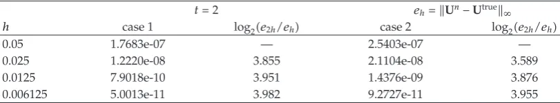
Table 1: Errors in max-norm for decreasinghand smooth analytical solution Utrue_{. Convergence rate} indicates a fourth-order convergence for the split scheme.

t2 ehUn_−Utrue

∞

h case 1 log₂e2h/eh case 2 log2e2h/eh

0.05 1.7683e-07 — 2.5403e-07 —

0.025 1.2220e-08 3.855 2.1104e-08 3.589

0.0125 7.9018e-10 3.951 1.4376e-09 3.876

0.006125 5.0013e-11 3.982 9.2727e-11 3.955

Table 2: Errors in max-norm for decreasinghand smooth analytical solution Utrue_{and using the non-split} scheme. Comparing withTable 1, we see that the splitting error is very small for this case.

t2,ehUn_−Utrue ∞

h case 1 case 2

0.05 1.6878e-07 2.4593e-07

0.025 1.1561e-08 2.0682e-08

0.0125 7.4757e-10 1.4205e-09

0.006125 4.8112e-11 9.2573e-11

5.2.2. Test example

For the first test case, we use a forcing function

fsint−xsiny−2μsint−xsiny−λμcosxcost−y sint−xsiny ,

sint−ysinx−2V s2sinxsint−y−λμcost−xcosy sinysint−y T, 5.10

giving the analytical solution

Utrue_{sinx−tsiny,siny−tsinx} T

. 5.11

Using the split method we solved2.4a on a domain x×y −11×−11 up tot 2. We used two sets of material parameters; for the first case ρ, λ, and μ were all equal to 1, for the second caseρ and μwere 1 andλ was set to 14. Solving on four different grids with a refinement factor of two in each direction between the successive grids we obtained the results shown in Table 1. The errors are measured in the ∞-norm defined as Uj,k maxmaxj,k|uj,k|,maxj,k|vj,k|. As can be seen we get the expected 4th order convergence for problems with smooth solutions.

To check the influence of the splitting error N4,θ on the error we solved the same problems using the non-split scheme3.11. The results are shown inTable 2. The errors are only marginally smaller than for the split scheme.

5.2.3. Singular forcing terms

fFδxgt, 5.12

where F is a constant direction vector. A numeric method for2.4aneeds to approximate the Dirac function correctly in order to achieve full convergence. Obviously we cannot expect convergence close to the source as the solution will be singular for two and three dimensional domains.

The analyzes in 13, 14 demonstrate that it is possible to derive regularized approximations of the Dirac function, which result in point wise convergence of the solution away from the sources. Based on these analyzes, we define one 2ndδh2and one 4thδ_h4

order regularized approximations of the one dimensional Dirac function,

δh2

x 1 h ⎧ ⎪ ⎪ ⎪ ⎨ ⎪ ⎪ ⎪ ⎩

1x, −h≤x < 0,

1−x, 0≤x < h,

0, elsewhere,

5.13

δh4x 1

h ⎧ ⎪ ⎪ ⎪ ⎪ ⎪ ⎪ ⎪ ⎪ ⎪ ⎪ ⎪ ⎪ ⎪ ⎪ ⎪ ⎪ ⎨ ⎪ ⎪ ⎪ ⎪ ⎪ ⎪ ⎪ ⎪ ⎪ ⎪ ⎪ ⎪ ⎪ ⎪ ⎪ ⎪ ⎩

111 6 x

5 8x

21

6x

3_{, −2h≤x < −h,}

11 2x−x

2₋ 1

2x

3_{, −h≤x < 0,}

1−1 2x−x

2 1

2x

3_{, 0≤x < h,}

1−11 6 xx

2₋1

6x

3_{, h≤x < 2h,}

0, elsewhere,

5.14

where in the above x x/h. The two and three dimensional Dirac functions are then approximated asδh2,4xδ _h2,4y andδ_h2,4xδ _h2,4yδ _h2,4z. The chosen time dependence was

a smooth function given by

gt ⎧ ⎨ ⎩ exp ₋₁

t1−t

, 0≤t <1,

0, elsewhere,

5.15

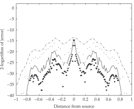
which is C∞. Using this forcing function we can compute the analytical solution by integrating the Green’s function given in 15 in time. The integration was done using numerical quadrature routines from Matlab. Figures11and12shows examples of what the errors look like on a radius passing through the singular source at timet 0.8 for different grid sizeshand the two approximationsδh2andδ_h4. As can be seen the error is smooth and

converges a small distance away from the source. However, usingδh2limits the convergence

to 2nd order, while usingδh4 gives the full 4th order convergence away from the singular

2-logarithm

o

f

|

err

o

r

|

−40 −35 −30 −25 −20 −15 −10 −5 0

Distance from source

−1 −0.8 −0.6 −0.4 −0.2 0 0.2 0.4 0.6 0.8 1

Figure 11: The 2-logarithm of the error along a line going through the source point for a point force located atx0,y0, and approximated in space by5.14. Note that the error decays asOh4_{away from the} source, but not near it. The grid sizes wereh0.05−·,0.025·,0.0125−,0.006125∗. The numerical quadrature had an absolute error of approximately 10−11 ≈2−36_{, so the error cannot be resolved beneath} that limit.

2-logarithm

o

f

|

err

o

r

|

−40 −35 −30 −25 −20 −15 −10 −5 0

Distance from source

−1 −0.8 −0.6 −0.4 −0.2 0 0.2 0.4 0.6 0.8 1

Figure 12: The 2-logarithm of the error along a line going through the source point for a point force located atx0,y0, and approximated in space by5.13. Note that the error only decays asOh2_{away from} the source. The grid sizes wereh0.05−·,0.025·,0.0125−,0.006125∗.

Dirac function. The convergence rate approaches 4 as we refine the grids, even though the solution was singular up to timet1.

Table 3: Errors in max-norm for decreasinghand analytical solution Utrue_{. Convergence rate approaches} 4th order after the singular forcing term goes to zero.

t1.1,ehUn_−Utrue ∞

h log₂e2h/eh

0.05 1.1788e-04 —

0.025 1.4146e-05 3.0588

0.0125 1.3554e-06 3.3836

0.00625 1.0718e-07 3.6606

0.003125 7.1890e-09 3.8981

smooth material properties, making the two methods roughly comparable in computational cost.

5.3. Three-dimensional test example for the elastic wave propagation

The motivation to compute also the three dimensional elastic wave propagation arose from the need to understand the anisotropy of the different dimensions, see2. We apply the three-dimensional model2.4a–2.4cfor our proposed splitting schemes.

5.3.1. The splitting scheme

In three dimensions a 4th order difference approximation of the right hand side operator becomes M4 ⎛ ⎜ ⎜ ⎜ ⎜ ⎜ ⎜ ⎜ ⎜ ⎜ ⎜ ⎜ ⎜ ⎜ ⎜ ⎜ ⎜ ⎜ ⎜ ⎜ ⎜ ⎜ ⎜ ⎜ ⎜ ⎜ ⎜ ⎜ ⎜ ⎜ ⎜ ⎜ ⎜ ⎝

λ2μ1− h

2

12D x2

Dx2

μ

1− h

2

12D y2

Dy2

1−h

2

12D z2

Dz2

λμ1−h

2

6D x2

D₀x

1−h

2

6 D y2

D₀y

λμ1−h

2

6 D x2

Dx₀

1− h

2

6 D z2

D₀z

λμ

1−h

2

6D x2

D₀x

1−h

2

6 D y2

D₀y

λ2μ

1−h

2

12D y2

Dy2

μ

1−h

2

12D x2

Dx2

μ

1− h

2

12D z2

Dz2

λμ

1− h

2

6 D z2

D₀z

1−h

2

6 D y2

Dy₀

λμ

1−h

2

6 D x2

Dx₀

1− h

2

6 D z2

D₀z

λμ

1− h

2

6 D y2

Dy₀

1−h

2

6 D z2

D₀z

λ2μ

1− h

2

12D z2

Dz2

μ

1−h

2

12D x2

Dx2

1−h

2

12D y2

Dy2

⎞ ⎟ ⎟ ⎟ ⎟ ⎟ ⎟ ⎟ ⎟ ⎟ ⎟ ⎟ ⎟ ⎟ ⎟ ⎟ ⎟ ⎟ ⎟ ⎟ ⎟ ⎟ ⎟ ⎟ ⎟ ⎟ ⎟ ⎟ ⎟ ⎟ ⎟ ⎟ ⎟ ⎠ , 5.16

operating on grid functions Un

j,k,l defined at grid points xj, yk, zl, tn similarly to the two dimensional case. We can splitM4into six parts;Mxx,Myy,Mzzcontaining the three second

There are a number of different ways we could split this scheme, depending on how we treat the mixed derivative terms. We have chosen to implement the following split scheme in three dimensions:

1 ρU

∗

j,k,l−2Unj,k,lUnj,k,l−1

Δt2 M4U

n

j,k,lθfnj,k,l1 1−2θfnj,k,lθfnj,k,l−1

2 ρU

∗∗

j,k,l−U∗j,k,l

Δt2 θMxx

U∗∗

j,k,l−2Unj,k,lUnj,k,l−1 θ 2

MxyMxz U∗

j,k,l−2Unj,k,lUnj,k,l−1

3 ρ

U∗∗∗

j,k,l−U∗∗j,k,l

Δt2 θMxx

U∗∗∗

j,k,l−2Unj,k,lUnj,k,l−1 θ 2

MxyMyz U∗∗

j,k,l−2Unj,k,lUnj,k,l−1

4 ρU n1

j,k,l−U∗∗∗j,k,l

Δt2 θMxx

Un1

j,k,l−2U n j,k,lU

n−1

j,k,l θ 2

MxzMyz U∗∗∗

j,k,l−2Unj,k,lU n−1

j,k,l . 5.17

The properties such as splitting error, accuracy, stability, and so forth, for the three dimensional case are similar to the two dimensional case treated in the earlier sections.

5.3.2. Testing the three dimensional scheme

We have done some numerical experiments with the three dimensional scheme in order to test the convergence and stability. We used a forcing

f−−1λ4μsint−xsinysinz−λμcosx2 sintsinysinzcostsinyz , −−1λ4μsinxsint−ysinz−λμcosy2 sintsinxsinzcostsinxz , −λμcost−ycoszsinx

−sinyλμcost−xcosz −1λ4μsinxsint−z T,

5.18

giving the analytical solution

Utrue_{sinx−tsinysinz,siny−tsinxsinz,sinz−tsinxsiny} T

. 5.19

As earlier we tested this for a number of different grid sizes. Using the same two sets of material parameters as for the two dimensional case we ran up untilt 2 and checked the max error for all components of the solution. The results are given inTable 4. We have also tested the three dimensional scheme using singular forcing functions approximated using 5.13 and 5.14. The results are very similar to the two dimensional case and we have therefore omitted them here.

6. Conclusion