Blaming the exogenous environment? Conditional efficiency estimation with continuous and discrete exogenous variables

Munich Personal RePEc Archive

Blaming the exogenous environment?

Conditional efficiency estimation with

continuous and discrete exogenous

variables

De Witte, Kristof and Mika, Kortelainen

University of Leuven (KUL), University of Manchester

4 March 2009

Online at

https://mpra.ub.uni-muenchen.de/14034/

Blaming the exogenous environment? Conditional

e¢ciency estimation with continuous and discrete

exogenous variables

Kristof De Witte

Centre for Economic Studies

University of Leuven (KU Leuven)

Naamsestraat 69, 3000 Leuven, Belgium

[email protected]

Mika Kortelainen

University of Manchester

Economics, School of Social Sciences

Oxford Road, Manchester, M13 9PL, UK

[email protected]

March 4, 2009

Abstract

This paper proposes a fully nonparametric framework to estimate relative e¢ciency of entities while accounting for a mixed set of continuous and discrete (both ordered and unordered) exogenous variables. Using robust partial frontier techniques, the prob-abilistic and conditional characterization of the production process, as well as insights from the recent developments in nonparametric econometrics, we present a generalized approach for conditional e¢ciency measurement. To do so, we utilize a tailored mixed kernel function with a data-driven bandwidth selection. So far only descriptive analysis for studying the e¤ect of heterogeneity in conditional e¢ciency estimation has been sug-gested. We show how to use and interpret nonparametric bootstrap-based signi…cance tests in a generalized conditional e¢ciency framework. This allows us to study statis-tical signi…cance of continuous and discrete exogenous variables on production process. The proposed approach is illustrated using simulated examples as well as a sample of British pupils from the OECD Pisa data set. The results of the empirical application show that several exogenous discrete factors have a statistically signi…cant e¤ect on the educational process.

Keywords: Nonparametric estimation, Conditional e¢ciency measures, Exogenous factors, Generalized kernel function, Education

JEL-classi…cation: C14, C25, I21

We would like to thank Laurens Cherchye and the participants of the Seminar on E¢ciency and Produc-tivity Analysis at Aston University for valuable comments.

1

Introduction

The traditional nonparametric procedures to estimate e¢ciency [such as the non-convex Free Disposal Hull (FDH; Deprinset al., 1984) and the convex Data Envelopment Analysis (DEA; Charnes et al., 1978)] have recently been directed towards the incorporation of exogenous environmental variables. Indeed, e¢ciency estimations which do not account for the oper-ational environment may have only a limited value. If, for example, the e¢ciency of the educational system is assessed, it is not fair or justi…ed to compare schools located in ‘good’ neighborhoods (e.g. measured by the highest degree of the mother, income of the parents, native language) with schools located in less advantageous areas. Thus, if the evaluated observations are a¤ected by external, exogenous factors, performance analysis should control for this heterogeneity.

The literature counts various approaches to incorporate the exogenous environment in nonparametric e¢ciency analysis (for an overview see Fried et al., 2008; for an extensive discussion see De Witte and Kortelainen, 2008). In general, the traditional approaches face one or several of the following drawbacks: (1) only either continuous or categorical exogenous variables can be used, (2) the e¤ect of environmental variable1 _{is required to be monotone in}

the production process (and possibly also concave if DEA is used), (3) the researcher has to choosea priori whether to model environmental variable as an input or as an output, (4) in practice it is often not possible to include several environmental factors, and (5) one needs to assume a separability condition in that the operational environment would not in‡uence the input or output levels, but only e¢ciency. Concerning the last drawback, obviously, in many applications the exogenous variables (e.g. the neighborhood and mother tongue) do in‡uence the observed input use (e.g. teaching hours) and output levels (e.g. test scores) of the observations. In this sense, there is no separability between the inputs and outputs on the one hand, and the exogenous variables on the other hand. Still, as the popular two-stage approach imposes separability assumption implicitly for all exogenous variables, its applicability in most applications is debatable.

Recently, Cazalset al. (2002) and Daraio and Simar (2005, 2007a) suggested a new ap-proach, which does not su¤er from the last four drawbacks. The approach starts from the probabilistic formulation of the production process and incorporates the operational environ-ment by conditioning on the exogenous characteristics. In particular, it limits the reference set of the evaluated unit by only comparing like with likes. This so-calledconditional e¢ciency

approach generalizes the traditional nonparametric approaches by avoiding the separability condition and by not requiring any speci…cation on the direction of in‡uence of exogenous variables. In addition, it allows one to include several environmental variables and to examine the e¤ect (favorable or unfavorable) of them. As the conditional e¢ciency approach avoids

the main disadvantages of the other models, it seems to be the most promising method to introduce external environmental factors into nonparametric frontier models. Therefore, the remainder of this paper concentrates on this approach.

Cazals et al. (2002) outlined the original idea on how to incorporate exogenous vari-ables in the non-convex nonparametric model. Daraio and Simar (2005, 2007a) expanded their approach to a more general multivariate (continuous) setup and presented a practical methodology to evaluate the impact of exogenous variables. Later, an extension to convex nonparametric models was proposed (Daraio and Simar, 2007b) and also a signi…cant amount of work has been done to prove the consistency and the asymptotic properties of di¤erent conditional e¢ciency estimators (Cazals et al., 2002; Jeonget al., 2008). As the merits of the approach are large (in particular avoiding the main drawbacks of the traditional proce-dures) it is increasingly used in several research questions. Previous applications include the productivity of universities (Bonaccorsi et al., 2006, 2007a, 2007b; Bonaccorsi and Daraio, 2008), e¢ciency in the water sector (De Witte and Marques, 2008; De Witte and Saal, 2008; De Witte and Dijkgraaf, 2009), performance of mutual funds (Daraio and Simar, 2005, 2006; Daouia and Simar, 2007; Jeonget al., 2008; Badinet al., 2008) and banks (Blass Staub and da Silva e Souza, 2007), e¢ciency of post o¢ces (Cazals et al., 2008), knowledge spillover and regional innovation performance (Bonaccorsi and Daraio, 2007c; Broekel, 2008; Broekel and Meder, 2008) and primary education (Cherchyeet al.,2007).

Nevertheless, some intricate issues remain. As the conditional e¢ciency approach relies on the estimation of nonparametric kernel functions to select the appropriate reference part-ners, it heavily relies on the choice of bandwidth parameters. The original article of Daraio and Simar (2005) considered the cross-validationk-nearest neighbor technique for estimating the bandwidths. However, besides being nonoptimal in …nite samples this bandwidth choice approach does not take into account the in‡uence of the exogenous variables on the produc-tion process. As such, although the condiproduc-tional e¢ciency estimates avoid the separability condition, their bandwidths relied on it. Recently, Badinet al. (2008) suggested an alterna-tive data-driven approach to select the optimal bandwidths. This approach accounts for the input and output variables while selecting values for the bandwidths. Moreover, following Hall et al. (2004), this data-driven procedure can help to identify external variables that have no in‡uence on the production process.

The current paper contributes to the literature by focusing on three additional issues, which are very relevant in most empirical applications. Firstly, it considers the inclusion of both discrete and continuous exogenous variables in the conditional e¢ciency framework. The conditional models used in previous studies have been designed for continuous environmental variables only.2 _{However, in interesting real-life applications the exogenous variables are}

both continuous and discrete. This paper shows how to adapt the nonparametric conditional e¢ciency measures to include mixed (i.e. both continuous and discrete) exogenous variables by specifying an appropriate kernel function which smooths the mixed variables. In doing so, we propose a procedure to estimate kernel bandwidths both for continuous and discrete variables (adapted from Hall et al., 2004). By estimating observation and variable speci…c bandwidths, our approach is able to estimate for every observation e¢ciency relative to a su¢ciently large reference group of similar units (i.e. units with a large probability of being similar).

Secondly, we argue and show that our approach can include a number of ordered and/or unordered categorical variables along with continuous exogenous variables even in relatively small samples. Related to this we know from previous research (Cazals et al., 2002; Jeong

et al., 2008) that the convergence rate of conditional e¢ciency estimators decrease when the number of continuous environmental variables increases. The typical curse of dimensional-ity in nonparametric models is deteriorated in the conditional e¢ciency models due to the smoothing on the exogenous variables. However, we show that this dimensionality problem is not the case for discrete exogeneous variables with compact support. In particular, we prove that the convergence rate of the proposed conditional e¢ciency estimator does not depend on the number of discrete variables. This is very relevant property in applications, because it allows one to include a large number of discrete environmental variables in conditional e¢ciency estimation without deteriorating accuracy of estimation.

Thirdly, we present a framework to test nonparametrically the signi…cance of the ex-ogenous variables. We note that, so far, only descriptive analysis for studying the e¤ect of the environmental variables in conditional e¢ciency estimation has been suggested (Daraio and Simar, 2005). This is in contrast to the two-stage semiparametric approach of Simar and Wilson (2007), which allows one to evaluate the signi…cance of exogenous variables in a second-stage truncated regression by the use of bootstrapping techniques. We extend the Daraio and Simar toolbox for visualizing the e¤ects of the continuous exogenous variables to a generalized setting which allows both visualization and statistical inference of continuous and discrete exogenous variables. For the signi…cance testing, we use recently developed nonparametric boostrap-based procedures. Thanks to our contributions, the nonparametric setup shares many bene…ts of a parametric model (i.e. multivariate analysis with continu-ous and discrete factors and with well established statistical inference), but without facing the major drawback of a parametric model (i.e. selecting a priori a functional form of the production process).3

many categories, since those variables are close to be continuous. Instead, the values of unordered discrete variables have no natural order, and thus cannot be modelled analogously with continuous variables.

3_{Nevertheless, if a parametric model is well speci…ed, the parametric estimator often has a higher rate of}

para-To illustrate our approach, we consider a couple of simulation scenarios that are similar to scenarios already used in the literature. However, in contrast to previous conditional e¢ciency studies, we study cases where univariate and multivariate exogenous factors can also include categorical components. To show potentiality of the approach in empirical applications, we demonstrate it by a relevant research question. In particular, the inclusion of both discrete and continuous exogenous variables in the conditional e¢ciency estimation is illustrated by assessing the e¢ciency of a random sample of British 15 years old pupils. We use the Pisa data set (Program for International Student Assessment) to estimate the performance of pupils while accounting for a broad range of unordered (e.g. mother tongue, possession of own room) and ordered (highest degree of mother and father) categorical and continuous (school size or teacher-student ratio) environmental variables. Including both discrete and continuous factors in the nonparametric model allows for a rich and solid analysis. Obviously, our approach is not limited to educational performance assessment but could be implemented in about all known applications.

The remainder of the paper unfolds as follows. Next section discusses the probabilis-tic formulation of the production process and describes the conditional e¢ciency approach. Section 3 presents our new approach based on generalized kernel estimation, its appropriate bandwidth selection and shows the procedure for testing the signi…cance of environmental variables. Section 4 illustrates the proposed method with a couple of simulated examples, while Section 5 applies the insights to the Pisa data set. Finally, we present the conclusions.

2

Conditional e¢ciency estimation

2.1

Probabilistic formulation and order-

m

Nonparametric e¢ciency measures are based on microeconomic production theory and esti-mation methods that do not require any functional form assumptions. In this framework it is typical to consider a production technology where production units are characterized by a set of inputsx(x2Rp+)and outputsy (y2R

q

+). The production technology is the set of of

all feasible input-output combinations: = (x; y) 2Rp++q jxcan producey . Obviously,

in practice the set and the e¢ciency measures are unknown and have to be estimated from a random sample of production units denoted by n =f(xi; yi)ji= 1; :::; ng.4

Besides above production set presentation, there exists alternative ways to describe gen-eral production processes. From alternative presentations, a probabilistic formulation of the

metric model delivers poor estimates in comparison to the nonparametric model.

4_{To clarify presentation, we denote the observed sample from which the e¢ciency scores are estimated by}

lowercase letters(xi; yi)whereas uppercase letters(X; Y)denote the unknown (and thus random) variables

production process presented …rst by Cazalset al. (2002) is particularly useful in many ap-plications. The idea behind this alternative formulation is to examine the probability that an evaluated observation(x; y)is dominated using the joint probability function:

HXY(x; y) = Pr(X x; Y y): (1)

Note thatHXY(x; y)is not a standard joint distribution function, because for the outputsy

the survival form is used, not the cumulative form like for the inputsx. The joint probability function can be further decomposed as (remark: we only present the output-orientation, for the input-orientation see Cazalset al., 2002):

HXY(x; y) = Pr(Y yjX x) Pr(X x)

=SYjX(Y yjX x)FX(X x)

=SY(yjx)FX(x) (in shorthand notation)

(2)

where SY(y j x) denotes the conditional survivor function ofY and FX(x)the cumulative

distribution function ofX:Now it can be shown that if is free disposal, the upper boundary of the support of SY(y j x) de…nes the traditional Farrell (1957) output-oriented technical

e¢ciency measure:

(x; y) = supf jSY( yjx)>0g= supf jHXY(x; y)>0g. (3)

This alternative presentation of the output-oriented e¢ciency score can be interpreted as the proportionate increase in outputs required for the evaluated unit to have zero probability of being dominated at the given input level.

To estimate e¢ciency scores using the probabilistic formulation, one needs to …rst sub-stitute the empirical distribution function HbXY;n(x; y) for HXY(x; y) and SbY;n(y j x) for

SY(yjx), correspondingly. These empirical analogs are given by:

b

HXY;n(x; y) = 1

n

n

X

i=1

I(xi x; yi y) (4)

and

b

SY;n(yjx) =

b

HXY;n(x; y)

b

FX;n(x)

= HbXY;n(x; y)

b

HXY;n(x;0)

; (5)

where I( ) is an indicator function. Using the plug-in principle, the Free Disposabal Hull (FDH) estimator for the output-oriented e¢ciency score can be then obtained asbF DH(x; y) =

supn jSbY;n( yjx)>0

o

.

It should be noted that the traditional FDH estimatorbF DH(x; y)has two major

constitute the production set: P rob((x; y) ) = 1. As such, the nonparametric technique is sensitive to outlying and atypical observations as these can heavily in‡uence the upper boundary of the support ofSbY;n(yjx):Therefore, Cazalset al. (2002) suggested to consider

the expected value of maximum output e¢ciency score of the unit (x; y), when compared to munits randomly drawn from the population of units using inputs less than the levelx. Thus, instead of considering the full frontier (or upper boundary), the idea is to draw a partial frontier depending on a random set of m variables which consume maximally xresources. Taking the expectation of this less extreme benchmark, we obtain the order-m e¢ciency measure m(x; y). If a unit is on average performing superior than its m randomly drawn

reference units (withX x), it obtains a ‘super-e¢ciency’ score (i.e. an output-e¢ciency score of m(x; y)<1) which is impossible in the traditional framework where by construction (x; y) 1. Cazals et al. (2002) showed that the order-m e¢ciency score m(x; y) has an

explicit expression that depends only on the conditional distributionSY(yjx):

m(x; y) =

R1

0 [1 (1 SY(uyjx))

m_{]du: (6)}

Similarly with FDH, one can then obtain the estimator for the order-m e¢ciency by plugging theSbY;n(yjx)to equation (6), which givesbm;n(x; y) =R₀1[1 (1 SbY;n(uyjx))m]du. Note

that this estimator is relatively easy to compute, as it based on a univariate integral. As shown by Cazals et al. (2002), the remarkable statistical property of the order-mestimator

bm;n(x; y)is its pn-consistency, i.e. it converges to the true value as quickly as parametric

estimators. Since this is valid for the general multiple input-output case, the estimator avoids the curse of dimensionality problem, which is very rare property for nonparametric methods.

2.2

Conditional order-

m

e¢ciency estimator

Z =z can be de…ned as:

HXYjZ(x; yjz) = Pr(X x; Y yjZ=z): (7)

Again, this can be further decomposed into:

HXYjZ(x; yjz) = Pr(Y yjX x; Z=z) Pr(X xjZ=z)

=SYjX;Z(Y yjX x; Z =z)FX(X xjZ=z)

=SY(yjx; z)FX(xjz): (in shorthand notation)

(8)

The support of SY(y j x; z) de…nes the production technology whenZ =z: To reduce the

deterministic nature, again instead of using the full support of SY(y j x; z) one can use

the expected value of maximum output e¢ciency score of the unit (x; y), when compared to m units randomly drawn from the population of units for which X x. Analogously to the unconditional order-m e¢ciencies, conditional e¢ciency measure m(x; yjz) can be

expressed using the following integral:

m(x; yjz) =

R1

0 [1 (1 SY(uyjx; z))

m_{]du: (9)}

EstimatingSY(yjx; z)nonparametrically is somewhat more di¢cult than for the

uncon-ditional case, as we need to use smoothing techniques in z (due to the equality constraint Z =z):

^

SY;n(yjx; z) =

Pn

i=1I(xi x; yi y)Kh(z; zi)

Pn

i=1I(xi x)Kh(z; zi)

; (10)

whereKh( )is a kernel function andhis an appropriate bandwidth parameter for this kernel.

The conditional order-m e¢ciency estimator ^m;n(x; y j z) is then obtained by plugging ^

SY;n(yjx; z)into equation (9), i.e.

^_{m;n(x; yjz) =}R1

0 [1 (1 S^Y;n(uyjx; z))

m_{]du: (11)}

Importantly, Cazalset al. (2002) showed that the convergence rate of estimatorbm;n(x; yj

z)depends on the dimension of Z, being (nhr₎ 1=2_{, where r = dim(Z).}5 _{This means that}

although order-mestimator avoids the curse of dimensionality, the accuracy of the conditional estimator depends on the dimension of Z due to the smoothing inz.

The current literature assumes that the univariate/multivariateZ is continuous. Clearly, an extension of the conditional e¢ciency approach to a more general setting including both discrete and continuous variables requires changes to the presented framework, because in

5_{Here it is assumed that bandwidth is similar for all environmental variables inZ. However, this}

general it is not appropriate to treat discrete variables similarly with continuous (i.e. use continuous kernel for all ordered and unordered discrete environmental variables). Next section discusses the treatment of discrete variables, the choice of kernel functions and the bandwidth selection in a generalized setting including both discrete and continuous exogenous variables.

3

Estimation with mixed data

3.1

Motivation

This section shows how to generalize the conditional e¢ciency approach to the case of mixed environmental factors (i.e. having both discrete and continuous components). Firstly, it is im-portant to notice that the conditional e¢ciency approach presented in Section 2 is similar to traditional nonparametric methods (like kernel methods) used in regression and density esti-mation with respect to the presumption that the underlying data is continuous. If one would have a data set containing a mix of continuous and discrete data, the conventional approach in nonparametric estimation would be to split the sample in subgroups (or ‘cells’) corresponding to the di¤erent values of the discrete variables and then estimate separate models/functions for those subsamples. This approach is sometimes referred to as a ‘frequency-based’ method. One could follow the frequency-based approach also in the conditional e¢ciency estimation by splitting the sample to subgroups with respect to the values of discrete variables, and then employ the methods presented in Section 2 for each of the subgroups (using inputs, outputs and continuous environmental variables). In essence, this would combine the conditional e¢ciency approach with a so-calledfrontier separation (ormetafrontier) approach.6

However, there are some important reasons why we do not see the sample splitting ap-proach very promising in conditional e¢ciency estimation. The …rst reason is that the frequency-based method will be problematic and even infeasible when the sample size is not large relative to the number of subgroups of discrete variables. For example, in our empirical application the sample size is 293, and the number of subgroups (or cells) is

6 6 3 2 16 = 3456 meaning that there are only 293=3456 0:08 observations per

subgroup on average! We note that this is not just a curious example; in fact, e¢ciency applications using parametric regression methods use frequently many discrete variables in relative small samples (100-300 observations). Besides the infeasibility problem, it is not practical to estimate a large number of models for di¤erent values of discrete variables. A

6_{An alternative framework for treating discrete environmental variables would be to ignore them in the}

further relevant disadvantage of the frequency-based method concerns statistical inference. Although it is is quite straigthforward to test the e¤ect of a dummy variable using boost-rapping methods by comparing e¢ciency distributions of separate groups, the test is much more challenging if there are more than two subgroups and in particular if one wants to test signi…cance of the categorical variable that has many classes.

To avoid the problems of the frequency-based method (as well as separability assumption), we propose to use an alternative approach that smooths also the discrete variables in a particular manner (as …rst suggested by Aitchison and Aitken, 1976). The idea of smoothing discrete along with continuous variables is based on novel kernel methods …rst presented by Qi Li, Je¤ Racine and their colleagues (see e.g. Racine and Li, 2004; Hall, Li and Racine, 2004; Li and Racine 2004, 2007, 2008). We introduce and adapt these techniques to conditional e¢ciency framework.

3.2

Generalized kernel estimation

As we treat continuous, discrete ordered (i.e. the discrete variables have a meaningful order) and discrete unordered variables (i.e. it does not matter how the variables are classi…ed to categories) di¤erently in the estimations, we rede…ne the multivariate Z. De…ne a vector of observed environmental variables byzi= (zic; zio; ziu), i= 1; :::; n, where the …rst component

zc

i 2Rrdenotes a vector of continuous environmental variables,zoi is av-dimensional vector

of environmental variables that assume ordered discrete values and zu

i is a w-dimensional

vector of exogeneous variables that assume unordered discrete values. In addition, let zo is

and zu

is denote sth components of zio and ziu. Without losing any generality, we assume

that zo

is andzisu can takecs 2 and ds 2 di¤erent values, i.e. ziso =f0;1; :::; cs 1g for

s= 1; :::; vandzu

is=f0;1; :::; ds 1gfors= 1; :::; w. This means that the support ofzoi and

zu

i areSo= v

Q

s=1f

0;1; :::; cs 1gandSu= w

Q

s=1f

0;1; :::; ds 1g, respectively.

To smooth both continuous and discrete variables, we use a standard multivariate product kernel for all three components in zi.7 By multiplying these multivariate kernel functions,

we obtain a generalized product kernel function, formally expressed as: Kh(z; zi) =

r Q s=1 1 hc s

lc z

c s zisc

hc s

r_Q+v

s=r+1

lo(zso; zois; hos) r+_Qv+w

s=r+v+1

lu(zsu; zisu; hus); (12)

wherelc_{( ),l}o_{( )andl}u_{( )are univariate kernel functions and h}c

s,hos andhus are bandwidths

for, respectively, continuous, ordered and unordered environmental variables. Regarding the continuous kernel function lc_{( ), we know from the previous research (Daraio and Simar,}

2005) that one should use kernels with compact support (i.e. kernels for whichk(z) = 0 if

jzj 1) such as the uniform, triangle, Epanechnikov or quartic kernels. In this study we will

7_{Of course, if any of the componentsz}c

i; zoi orziuis univariate, then an univariate kernel su¢ces for that

use the Epanechnikov kernel (although other compact kernels deliver very similar results). For unordered variables we employ the Aitchison and Aitken (1976) discrete univariate kernel function that was designed for discrete variables without any order, while for ordered dis-crete variables we employ the Li and Racine (2007) disdis-crete kernel function that also takes into account the ordering of the categories. Formally, these continuous and discrete kernel functions are given by:

lc z

c s zcis

hc s = 8 > < > : 3 4p5 1

1 5 zc s z c is hc s 2

if zcs z c is hc s 2 5 0 otherwise (13)

lu(zus; zuis; hus) =

(

1 hu

s ifzisu =zus

hu

s=(cs 1) ifzisu 6=zus

(14)

lo(zso; ziso; hos) = (hos)jz

o

is zsoj: (15)

It is worth considering the two discrete kernel functions in more detail, as they have not been previously used in nonparametric e¢ciency literature. Firstly, both the Aitchison and Aitken (1976) and Li and Racine (2007) kernel functions impose contraints for bandwidth parameters. For the former, bandwidth hu

s must be between 0 and (cs 1)=cs, whereas

for the latter bandwidth ho

s can take values between [0,1].8 By considering the limit

val-ues ofhu

s, we see that whenhus = 0 then lu(zus; zuis;0) = I(zisu =zsu) becomes an indicator

function, while hu

s = (cs 1)=cs giveslu(zsu; zisu;(cs 1)=cs) = 1=cs, i.e. a constant

ker-nel function. The …rst special case is of particular interest, because the indicator function divides the sample to subgroups exactly the same way as the frequency-based method dis-cussed in Section 3.1. Similarly, we can observe that when ho

s = 1, Li and Racine kernel

function becomes lo_(zo

s; zois; hos) = 1for all values ofzso andziso 2 f0;1; :::; cs 1g such that

the irrelevant variable zo

s will be smoothed out. In our conditional e¢ciency setting, the

discrete kernel estimations boil intuitively down to in the order-m estimation drawing with a nonnegative probability of (1 hu

s) observations which belong to the same class as the

evaluated observation, and with a nonnegative probability of hu

s=(cs 1) (or alternatively

for unordered variables(hos)jz o

is zosj)observations which do not belong to this class. Drawing

observations which both belong to and not belong to the evaluated class (although with a di¤erent probability) smooths the discrete variable.

Having presented the idea of smoothing the mixed variables with the generalized kernel approach, we apply the technique to the conditional e¢ciency framework. For multivariate z = (zc_{; z}o_{; z}u_{) including continuous and unordered and ordered discrete components, the}

8_{For example, if we have an unordered dummy variable, we know thatc}

estimator for the conditional survivor function ofY can be expressed as:

b

SY;n(yjx; z) =

Pn

i=1_PI(xi x; yi y)Kh(z; zi)

n

i=1I(xi x)Kh(z; zi)

; (16)

where Kh(z; zi) is the generalized multivariate kernel function speci…ed in equation (12).

Further, one can again obtain the conditional e¢ciency estimator bm;n(x; yjz)by plugging

in SbY;n(yjx; z)in equation (6).

To show the validity of the approach, and in particular to show the consistency of the estimators, we make the following assumptions.

Assumption (A1): The sample observations Sn = f(xi; yi; zi)ji= 1; :::; ng are

real-izations of independent and identically distributed (iid) random variables(X; Y; Z)with the probability density functionfXY Z(x; y; z). Both the marginal density functionfZ(z)and the

conditional survivor function SY(y j x; z) have continuous second order partial derivatives

with respect to zc_{. For …xed values ofx; y andz,f}

Z(z)>0and0< SY(yjx; z)<1:

Assumption (A2): lc_{( )is a symmetric, bounded, and compactly supported density}

function.

Assumption (A3): Asn! 1,hc

s!0fors= 1; :::; r,hos!0 fors= 1; :::; v,hus !0

fors= 1; :::; w, and(nhc

1hc2:::hcr)

1 2 ! 1.

The following theorem and corollary give the convergence rate of SbY;n(y j x; z) and

bm;n(x; yjz).

Theorem 1 Under Assumptions (A1) to (A3), SbY;n(y jx; z)converges to SY(yjx; z) with

O_{p (nh}c_1hc_2:::hc_r) 12 _:

Proof.

First, note that we can write the conditional survivor function estimator as:

b

SY;n(yjx; z) =

P

i2N_PxI(yi y)Kh(z; zi) i2NxKh(z; zi)

; (17)

where Nx = fxijI(xi x) = 1,i= 1; :::; ng. Li and Racine (2008) prove that FbY;n(y j

z) =

Pn

i=1_PI(yi y)Kh(z; zi)

n

i=1Kh(z; zi)

converges to FY(y j z) in mean square error (and hence

in probability) with O_{p (nh}c

1hc2:::hcr)

1

2 _{under regularity conditions that are similar to}

Assumptions (A1)-(A3). Besides X x, the only di¤erence to Li and Racine (2008) is that we are estimating the conditional survivor functionSY(yjz)instead of the conditional

distribution functionFY(y jz). Since by de…nition SY(yj z) = 1 FY(y jz), their results

extends to our case when condition onX x:

The following result follows directly from Theorem 1, as for givenm m(x; yjz)depends

Corollary 1 Under Assumptions (A1) to (A3),bm;n(x; yjz)converges to m(x; yjz) with O_{p (nh}c

1hc2:::hcr)

1

2 _{for any …xed value of m.}

These results prove that the conditional e¢ciency estimatorbm;n(x; yjz)is consistent in

a more general case including both discrete and continuous environmental variables. Addi-tionally, they show that the convergence rate of the estimator is(nhc

1hc2:::hcr)

1

2_{, i.e. it does}

not depend on the number of discrete variables inZ but only on the number of continuous variables. This is very relevant result, since e¢ciency applications use frequently several discrete exogenous factors in small samples.

3.3

Bandwidth selection: A data-driven method

The bandwidth selection is the most crucial step in nonparametric kernel estimation (cfr. it has almost the same importance as the model speci…cation in parametric estimations). If the bandwidth is too large, the kernel function will be oversmoothed; if the bandwidth is too small, the kernel function will be undersmoothed. The initial proposal of Daraio and Simar (2005) estimated forzc_{the bandwidthsh}c _{by the likelihood cross-validationk-nearest}

neighbor technique. However, only asymptotic optimality of this approach has been shown and although the conditional e¢ciency estimates try to avoid the separability condition, its bandwidth selection relies on it. Indeed, by only relying on the exogenous variables, the estimation ofhc _{ignores the impact ofz}c _{on the production process (i.e. the impact ofz}c _on

y given thatxi x). Therefore, conditional bandwidth estimations are required.

Similar as before, the main challenge lies in extending the traditional bandwidth estima-tions for y conditional on Z =z, to estimations for y conditional on X xand Z =z (as required by the conditional e¢ciency model). The former conditional bandwidth estimations are developed by the models of Hallet al. (2004) and Li and Racine (2007, 2008). The latter conditional e¢ciency estimations are explored by Badinet al. (2008) for continuous variables only. Following the lines of Badin et al. (2008) we adopt the approach of Hall et al. (2004) to our framework.

To estimate bandwidths(hc_{; h}o_{; h}u_{), we minimize the cross-validation functionCV(h}y_{; h}c_{; h}o_{; h}u_),

where hy _{is a bandwidth vector for outputs y:Note that although we estimate bandwidths}

also for y, those bandwidths are not used in conditional e¢ciency estimation.9 _De…ne

therefore the conditional PDF of Y for X x and Z = z (with z = (zc_{; z}o_{; z}u_{)) as}

g(y j X x; Z = z) = f(y; X x; Z = z)=m(X x; Z = z) where f denotes the joint density of (y; z) and m the marginal density of z for given X x: The density f and the marginal density m are not observed but can be estimated by the use of nonnegative, generalized kernelsK( )andL( ):

^

f(y; xi x; z) = 1_nPni=1I(xi x)Kh(z; zi)Lhy(y; yi) ^

m(xi x; z) =_n1Pn_i=1I(xi x)Kh(z; zi)

(18) where the generalized kernelKh(z; zi)is computed as in equation (12) and the multivariate

kernelLhy(y; yi)as

Qq j=1

1

h_yjl yj yij

h_yj withl( )a univariate kernel function (Epanechnikov).

We start from the weighted integrated squared error (ISE) betweeng^( )andg( ): ISE =R f^g(yjxi x; z) g(yjxi x; z)g2m(xi x; z)dW(z)dy

=R^g(yjX x; z)2_m(x

i x; z)dW(z)dy (I1n)

2Rg^(yjX x; z)g(yjX x; z)m(xi x; z)dW(z)dy (I2n)

+Rg(yjX x; z)2_m(x

i x; z)dW(z)dy (I3n)

(19)

wheredW(z)denotes an in…nitesimal element of a measure (in order to avoid for the continu-ous components ofz,zc_{, dividing by 0 in the ratiof^(y; x}

i x; z)=m^(xi x; z)):The leading

term of theISE (i.e. the part depending on the bandwidth; which corresponds in equation (19) with the terms I1n and I2n as these have estimates ofg( )) can be approximated by a

cross-validation (CV) objective function which does not use numerical integration, nor initial assumptions on bandwidths or density function estimators. Hallet al. (2004) show that the leading term of theCV criterion corresponds to:

CV(hy₁; :::; hy

q; hc1; :::; hcr; ho1; :::; hov; hu1; :::; huw) = ^I1n 2 ^I2n (20)

where the empirical approximations ofI1n andI2n, respectively, I^1n and I^2n;are based on

a leave-one-out sample, i.e. a sample of (n 1) observations due to deleting observation i from the sample. By optimizing (hy1; :::; hyq; hc1; :::; hcr; ho1; :::; hov; hu1; :::; huw), we minimize the

CV function.

It can be shown that the optimal order of the bandwidths corresponds hc

s n 1=(5+r)

andho;u

s n 2=(5+r) (Li and Racine, 2008). However, as we basically estimate the optimal

bandwidth for the conditional PDF instead of for the closely related conditional CDF, we

9_{In total, there areq+r+v+wbandwidths:(h}y_{; h}c_{; h}o_{; h}u_{) = (h}y 1; :::; h

y

q; hc₁; :::; hcr; ho1; :::; hov; hu1; :::; huw),

need to adjust the bandwidths to obtain bandwidths of the optimal order ofhc

s n 1=(4+r)

and ho;u

s n 2=(4+r). The bandwidths as computed along the conditional PDF can be

corrected by multiplyinghc swithn

1 5+r

1

4+r andho;u s byn

2 5+r

2 4+r.

As also remarked by Badinet al. (2008, p. 8), the only di¤erence between the general-ized conditional bandwidth computation of Hall et al. (2004) and the optimal data-driven bandwidth needed for the conditional e¢ciency framework is the reduction of the reference sample size where(hc_{; h}o_{; h}u_{)are computed in. In particular, instead of using the full}

refer-ence sample (consisting ofnobservations) we only consider the observations for whichxi x

and compute for this limited reference set the bandwidths (hc_{; h}o_{; h}u_{). As such, we obtain}

for every observation a particular set of bandwidths in each of its dimensions (i.e. for every element ofzi). As a disadvantage, this approach dramatically limits the number of reference

units for observations with a smallx.10

Finally, we note that in some applications one might want to compare performance of units only with the observations in the same category (i.e. the same value of discrete vari-able). For example, in evaluating e¢ciency of hospitals using data from several countries, one may want to limit comparison units to hospitals in the same country because of the technological and operational di¤erences. In our framework this is very easy to implement by imposing bandwidth to be zero for the discrete variable in question (i.e. country). It is worth emphasizing that the presented framework still allows bandwidths of other discrete en-vironmental variables to be positive and in that sense is more general than the nonparametric frequency-based (or frontier separation) approach.

3.4

Examining the in‡uence of exogenous variables on the

produc-tion process

3.4.1 Visualization

To evaluate systematically the in‡uence of exogeneous variables on the production process, we can compare the conditional e¢ciency measure bm;n(x; y j z) with the unconditional

e¢ciency measurebm;n(x; y):In particular, we follow the methodology suggested by Daraio

and Simar (2005, 2007a) by nonparametrically regressing the ratio of the conditional and unconditional e¢ciency measure Qz ₌ bm;n(x;yjz)

b_m;n(x;y) on environmental factors z. They use a

smooth nonparametric kernel regression to estimate the modelQz

i =f(zi) + i. In addition,

they visualize the estimated relationships between environmental variables and the ratio of e¢ciency scores. Using simulations, Daraio and Simar showed that this approach allows one to detect positive, negative, neutral or even nonmonotone e¤ects of the environmental factors on the production process.

WhenZ is continuous and univariate the visualization is straigthforward as one can use scatterplots ofQz_{againstZ;and as a smoothed nonparametric regression curve can illustrate}

the e¤ect ofZ onQz_{. For example in an output-oriented e¢ciency, a horizontal line implies}

thatZ does not a¤ect the production process, whereas an increasing (decreasing) smoothed regression curve shows that Z is favorable (unfavorable) to the production process. By interpretation, a favorable e¤ect means that the environmental variable plays the role of a ‘substitutive’ input in the production process by increasing the productivity of traditional inputs, whereas an unfavorable e¤ect implies that the environmental variable contraints the production by using more inputs in production activity.

WhenZ is multivariate and includes also discrete variables, visualization is also feasible, although somewhat more challenging. For dim(Z) = 2, one can use 3-dimensional plots. However, ifdim(Z)>2, those are not enough. Perhaps the easiest solution for multivariate cases is to examine so-calledpartial regression plots (see e.g. Daraio and Simar, 2007a; Badin

et al., 2008), where only one (or two) environmental variable(s) is (are) allowed to change and other variables are kept at a …xed value. Further, one can then use several di¤erent …xed values such as median and 1st and 3rd quartile to examine whether the e¤ect on individual variableZsis the same for di¤erent values of others exogenous factors. This kind

of procedure helps to recognize the e¤ect of individual variable on the production process and possible interactional e¤ects between environmental variables. Moreover, it can be used also for discrete variables as we illustrate in the empirical application.

3.4.2 Nonparametric estimation and inference

Although it can be useful to visualize the e¤ect of environmental variables on the production process, researchers are usually more interested in their statistical signi…cance. Yet in the conditional e¢ciency framework, so far, only descriptive analysis has been suggested and applied in studying the e¤ect of environmental variables on the production process. This is in sharp contrast to the papers using two-stage models, where tools of statistical inference have been used extensively. Our aim is to propose for robust conditional e¢ciency models a framework to test the signi…cance of mixed multivariate environmental variables in the production process. We follow the lines of earlier research by focusing on smoothed nonpara-metric regression. However, instead of Nadaraya-Watson kernel regression, which has been mostly used in previous conditional e¢ciency studies, we will use local linear regression for estimating Qz

i =f(zi) + i. Compared to the Nadaraya-Watson kernel estimator (i.e. local

constant regression), the local linear estimator is less sensitive to boundary e¤ects and can also simultaneously uncover the marginal e¤ects of the environmental variables onQz_.11

As in our frameworkZcan include both discrete and continuous variables, it is again useful

to employ smoothing techniques which allow one to estimate the nonparametric regression model without sample splitting (i.e. which was the case in the frequency-based approach). Therefore, we use the nonparametric regression method developed by Racine and Li (2004) and Li and Racine (2004), which smooths both continuous and discrete variables. To present the basic idea shortly, consider our nonparametric model:

Qzi =f(zi) + i; i= 1; :::; n (21)

where as previously Qz i =

b_m;n(xi;yijzi)

b_m;n(xi;yi) , zi = (z c

i; zio; ziu) includes values of continuous,

or-dered and unoror-dered exogenous variables for observation i, i is the usual error term with

E(ijzi) = 0, andf is the conditional mean function. The local linear method is based on

the following minimization problem:

min

f ; g

n

X

i=1

(Qzi (zic zc) )

2

Kh(z; zi); (22)

whereKhis the generalized product kernel function de…ned earlier. Lettingb=b(z)andb=

b(zc_{)denote the solutions that minimize equation (22), it is straigthforward to show that local}

linear estimators b(z) and b(zc_{) are consistent estimators for f(z) =E(Q}z_{jz) and (z}c_):

Note that the practical advantage of local linear regression is the fact that one can estimate simultaneously both the conditional mean function f(z) and the gradient vector (zc_{) for}

continuous components (which can be interpreted as varying coe¢cient). For bandwidth choice we use again the least-squares cross-validation, although one can employ also other methods available in literature.

Since our estimation framework is fully nonparametric, we also want to avoid any paramet-ric assumptions in the statistical inference stage.12 _{It is worth emphasizing that parametric}

assumptions would be di¢cult to justify in this context and even inconsistent with our non-parametric e¢ciency estimation. Thus, to test the signi…cance of regressors in (21), we will utilize recently developed nonparametric tests. More speci…cally, we test the signi…cance of each of the continuous and each of the discrete variables using tests, respectively, proposed by Racine (1997) and Racine et al. (2006). These tests can be seen as the nonparametric equivalent of standard t-tests in ordinary least squares regression. However, nonparametric test are more general than standardt-tests, as the former tests both linear and (unspeci…ed) non-linear relationships. In a multivariate setting the null hypotheses for testing continuous

1 2_{Note that our robust conditional e¢ciency framework does not su¤er from the statistical problems of}

and discrete (both ordered and unordered) components are, respectively:

H0 : E Qz Z; Ze sc =E Qz Ze almost everywhere, and (23)

H0 : E Qz Z; Ze sd =E Qz Ze almost everywhere, (24)

where Zc

s andZsd denote sth component of continuous and discrete (ordered or unordered)

variables and Ze represent all other environmental variables, which can be both continuous and discrete. The alternative hypotheses H1 are negations for the null hypotheses. Thus,

e.g., for the second case the alternative hypothesis isH1:E Qz Z; Ze sd 6=E Qz Z :e

To deduce a practical implementation, we …rstly rewrite the null hypothesis for continuous variables as:

H0:

@E Qz _{Z; Ze} c s

@Zc s

= (Zsc) = 0almost everywhere; (25)

i.e., that the partial derivative off(Z)with respect toZc

s is zero. Using this representation,

the test statistic for continuous components can be written as:

Ic=En (Zsc)

2o

: (26)

A consistent estimator for this test statistic can be obtained by substituting the local linear estimator for unknown derivative and using a sample average ofI, i.e.

Inc = 1

n

n

X

i=1

b(zis)2: (27)

To estimate the …nite-sample distribution and critical value of the test statisticIc

n,

nonpara-metric bootstrap procedures can be used. We shortly explain the steps of the bootstrap procedure; for more details, see Racine (1997). First estimate the conditional mean function E Qz _{Z; Ze} c

s f0 and save residualsbi; i= 1; :::; n:Secondly, resample with replacement

from the residual distributionF ;b which has probability mass 1

n for allbi;to obtain a

boot-strap samplefbig n

i=1:Thirdly, generate a bootstrap sample

n b

Q_i; zi

on

i=1, whereQbi = ^f 0

i +bi;

i= 1; :::; nandzi include all conditioning variables. Fourthly, estimateb(zis) and the test

statistic using the bootstrap sample. By repeating steps (1)-(4)B times (whereB is a large number) one obtains a sample distribution that can be then used for calculating critical values andp-values for the test statistic.

Secondly, for discrete variables a statistic similar to (27) can be used for the signi…cance testing. Let us assume that the testable discrete variableZd

s (ordered or unordered) takesc

di¤erent values, f0;1;2; :::; c 1g. If we denote the conditional mean function by f(Z; Ze d s);

the null hypothesisE Qz _{Z; Ze} d

s =E Qz Ze is equivalent tof(Z; Ze sd=l) =f(Z; Ze sd= 0)

Id= c 1

X

l=1

E hf(Z; Ze sd=l) f(Z; Ze sd= 0)

i2

; (28)

which is clearly always nonnegative and equals zero when the null hypothesis is true. A consistent estimator of the test statistic is then obtained as:

Ind= 1

n

n

X

i=1

c 1

X

l=1

h b

f(zei; zisd =l) fb(zei; zdis= 0)

i2

; (29)

wherefbis the local linear estimator of the conditional mean function at the given values of the variables. This estimator can be straightforwardly generalized also to the case, where multiple discrete variables are tested simultaneously.

To approximate the …nite-sample distribution of Id

n, we will again use a boostrap

pro-cedure.13 _{As the procedure is a bit di¤erent than for continuous variables, we next sketch}

shortly the steps. Firstly, randomly select zisd; from zisd n

i=1 with replacement and call

n b

Qi;ezi; zisd;

on

i=1 the bootstrap sample. Secondly, use the bootstrap sample to compute the

bootstrap statistic I ;d

n , which is otherwise similar than (29) but zdis is replaced by z d; is :

Thirdly, by repeating steps 1 and 2 B times (withB a large number) one obtains a sample distribution that can be then used for calculating critical values and p-values.

4

Numerical illustrations

To illustate the proposed methods, we next present some examples using simulated data sets. We followed earlier literature by considering a simulated output-oriented model with multiple inputs and multiple outputs. The data generating process is similar as in Parket al.

(2000), Daraio and Simar (2005, 2007) and Badinet al. (2008). However, although inputs and input-output relationships were generated similarly, we deviate from previous conditional e¢ciency studies by allowing Z to include also discrete exogenous factors. To this end, we …rst consider an example including univariate discreteZ and then cases with multivariateZ including both discrete and continuous components.

All the examples concentrate on a two-input and two-output technology, which is repre-sented by the following convex technology:

y(2) = 1:0845 x(1) 0:3 x(2) 0:4 y(1) (30) where y(1)_{; y}(2)_{; x}(1) _{and x}(2) _{denote the …rst and the second components of outputs and}

inputs, respectively. We generate independent uniform variables using X_i(j) U(1;2) and

1 3_{Note that Racineet al. (2006) propose for discrete variables also two alternative bootstrap procedures}

e

Y_i(j) U(0:2;5)forj = 1;2. The output e¢cient random points, which do not include yet the e¤ect ofZ, are calculated by:

Y_{i;ef f}(1) =1:0845 X

(1) 0:3 _X(2) 0:4

Si+ 1

(31) Yi;ef f(2) = 1:0845 X(1)

0:3

X(2)

0:4

Yi;ef f(1) ; (32)

where Si = Yei(2)= Ye

(1)

i represent the slopes which characterize the generated random rays

in the output space for j = 1;2. Output values are then generated by multiplying the output e¢cient random points by an ine¢ciency termexp (Ui);whereUi Exp(1=3);and

by terms representing the e¤ect of exogenous variables Z. In all simulations, we use the following formulas to specify the dependency on environmental factors:

Y_i(1)=Y_{i;ef f}(1) (1 + 1Z1;i) (1 + 2Z2;i) (1 + 3Z3;i) (1 + 4Z4;i) exp (Ui); (33)

Y_i(2)=Y_{i;ef f}(2) (1 + 1Z1;i) (1 + 2Z2;i) (1 + 3Z3;i) (1 + 4Z4;i) exp (Ui); (34)

where Z1;i 2 f0;1;2g with P(Z1;i=l) = 1=3 for l = 0;1;2; Zt;i 2 f0;1g for t = 2;3

with P(Zt;i=l) = 0:5 for l = 0;1; and Z4;i N(10;3): The values of coe¢cients t

for t = 1;2;3;4 are speci…ed separately for di¤erent simulations. We treat all the discrete variables as unordered and thus use Aitchison and Aitken kernel function for them, while Epanechnikov kernel is employed for continuous variable (see Section 3.2). Finally, for each case we simulate a sample of n= 100observations and selectm= 30andB= 1000.

Simulated case 1: univariate discrete Z

In the …rst case, we set in equations (33) and (34) 1 = 1:2 and 2 = 3 = 4 = 0, which

givesYi(j)=Y

(j)

i;ef f (1 + 1:2Z1;i) exp (Ui)forj= 1;2. In other words, in this univariate case

Simulated case 2: multivariate mixed Z

In the second case, we set 1= 1:2, 2= 0:5; 3= 1 and 4= 1such that we include three

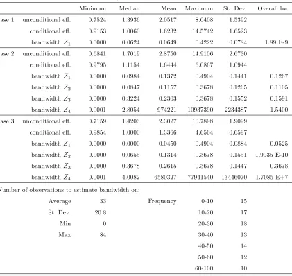
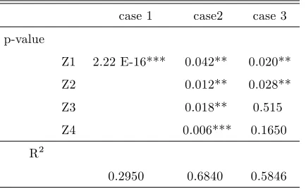
(unordered) discrete and one continuous exogenous variables in the data generating process and in estimation. The results, as presented in Tables 1 and 2 again show the appropriate working of the model. Indeed, as in the simulation each of the exogenous variables (positively) in‡uence outputs, we correctly observe low median bandwidths. This is also re‡ected in the low (and thus highly signi…cant) p-values of the test statistic. Interestingly, the bandwidth values of Z4are very large for some of the observations, which explain the high mean value.

However, this is only case for a small number of observations (see median value), and the e¤ect of Z4is anyway signi…cant.

Simulated case 3: insigni…cant variables

In the last scenario, we test for the inclusion of irrelevant variables in the model. Therefore, we set 1 = 1:2, 2 = 0:5; 3 = 0 and 4 = 0, in which case Z3 and Z4 are generated

independently on inputs and outputs having no in‡uence on the production process. In contrast to the …rst case we now use all the exogenous variables to examine whether our method can recognize insigni…cant variables (i.e. Z3 andZ4). The results in Tables 1 and 2

show that this is indeed the case, as the irrelevant in‡uence is con…rmed by the high p-values of the nonparametric tests for Z3 and Z4. However, one should note that the observation

speci…c median bandwidths forZ3 and especially forZ4 have not increased a lot. The …rst

of these can be explained by the fact that median bandwidth forZ3actually equals its upper

bound (0.50) before the correction ofn5+2r 2

4+r. For continous variable the median bandwidth

is instead quite far from what we would expect. On the other hand, remark that the overall (non-observation speci…c) bandwidths capture correctly the in‡uence of Z1 andZ2 and the

non-in‡uence of Z3 and Z4. Based on these simulation results it seems that observation

speci…c bandwidths are not so powerful in recognizing insigni…cant variables than the overall bandwidths. This might be explained by the sample sizes used in bandwidth estimations; while the bandwidth choice in conditional e¢ciency estimation uses less than 30 observations for a half of the sample, the overall bandwidths are based on the whole sample. In any case, this example shows that it is not necessarily enough to consider only observation speci…c bandwidth values when examining the statistical signi…cances of exogenous variables, but also statistical inference tools (and / or not observation speci…c bandwidths) are needed. However, we leave a more detailed examination of this issue for further research.

Table 1: E¢ciency estimates and bandwidths

Minimum Median Mean Maximum St. Dev. Overall bw case 1 unconditional e¤. 0.7524 1.3936 2.0517 8.0408 1.5392

conditional e¤. 0.9153 1.0060 1.6232 14.5742 1.6523

bandwidthZ1 0.0000 0.0624 0.0649 0.4222 0.0784 1.89 E-9

case 2 unconditional e¤. 0.6841 1.7019 2.8750 14.9106 2.6730 conditional e¤. 0.9795 1.1154 1.6444 6.0867 1.0944

bandwidthZ1 0.0000 0.0984 0.1372 0.4904 0.1441 0.1267

bandwidthZ2 0.0000 0.0847 0.1157 0.3678 0.1265 0.1105

bandwidthZ3 0.0000 0.3224 0.2303 0.3678 0.1552 0.1591

bandwidthZ4 0.0001 2.8054 974221 10937390 2234387 1.5400

case 3 unconditional e¤. 0.7159 1.4203 2.3027 10.7898 1.9099 conditional e¤. 0.9854 1.0000 1.3366 4.6564 0.6597

bandwidthZ1 0.0000 0.0000 0.0450 0.4904 0.0884 0.0525

bandwidthZ2 0.0000 0.0655 0.1314 0.3678 0.1551 1.9935 E-10

bandwidthZ3 0.0000 0.3678 0.2615 0.3678 0.1447 0.3678

bandwidthZ4 0.0001 4.0082 6580327 77941540 13446070 1.7085 E+7

Number of observations to estimate bandwidth on:

Average 33 Frequency 0-10 15

St. Dev. 20.8 10-20 17

Min 0 20-30 18

Max 84 30-40 13

40-50 14 50-60 12 60-100 10

to a real life data set.

5

Application to educational e¢ciency

5.1

The performance of pupils

Table 2: Nonparametric signi…cance test

case 1 case2 case 3 p-value

Z1 2.22 E-16*** 0.042** 0.020** Z2 0.012** 0.028** Z3 0.018** 0.515 Z4 0.006*** 0.1650 R2

0.2950 0.6840 0.5846

where "***" denotes signi…cance at 1% level, "**" at 5% and "*" at 10%.

discrete and continuous variables is particularly valuable when assessing educational data.14

We estimate the performance of British pupils at the age of 15 as surveyed by the inter-national Pisa (Program for Interinter-national Student Assessment) data set for 2006. The latter OECD survey is currently at its third wave (2000, 2003 and 2006) and contains survey data for more than 400,000 pupils from 57 countries. Besides a pupil survey, it consists of a survey by the school and by the parents which try to capture the socio-economic background of the pupil. We limited our sample to 16 randomly chosen English and Welsh schools which count in total 293 surveyed pupils. By considering a small sample, we try to illustrate that our conditional e¢ciency approach is able to include a large number of discrete variables without losing accuracy of the estimation. As the conditional e¢ciency model relies on the robust e¢ciency estimates, it is also well suited to deal with the extremal and atypical observations which could arise from survey data (e.g. Boundet al., 2001).

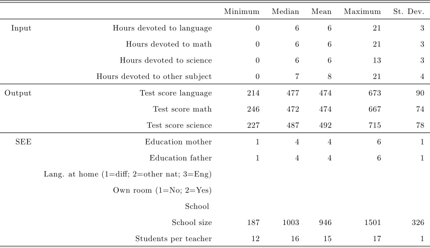
The conditional order-m estimation requires the selection of input, output and environ-mental variables. We follow the education literature in selecting these. Students are spending resources (in particular time) to study languages, math, science and other skills. The four input variables sum for, respectively, language, math, science and other subjects the total hours that pupil reported to spend on the subject during regular classes, out of school and self study (i.e. the sum of the variables ST31Q in the Pisa data set). As such, the inputs proxy the devotion to the subjects. Given these e¤orts, students are obtaining test results which are proxied by 5 plausible values for, respectively, language, math and science (the plausible values are standardized across the OECD countries with an average score of 500). Following the standard literature (e.g. OECD, 2007) we consider as output variables the arithmetic average of the 5 plausible values in the Pisa data set for each of the three

sub-1 4_{Obviously, the scope of the generalized conditional e¢ciency framework is much broader. Therefore, the}

Table 3: Descriptive statistics

Minimum Median Mean Maximum St. Dev. Input Hours devoted to language 0 6 6 21 3 Hours devoted to math 0 6 6 21 3 Hours devoted to science 0 6 6 13 3 Hours devoted to other subject 0 7 8 21 4 Output Test score language 214 477 474 673 90 Test score math 246 472 474 667 74 Test score science 227 487 492 715 78 SEE Education mother 1 4 4 6 1 Education father 1 4 4 6 1 Lang. at home (1=di¤; 2=other nat; 3=Eng)

Own room (1=No; 2=Yes) School

School size 187 1003 946 1501 326 Students per teacher 12 16 15 17 1

jects. The socio-economic environment (SEE) of the pupil is captured by 7 environmental variables (following Hampden-Thompson and Johnston, 2006 and references therein). We include two ordered variables, i.e. the education of the mother and the father as proxied by a variable between 0 (did not complete ISCED 1; where ISCED denotes the International Standard Classi…cation of Education by the Unesco) and 6 (completed ISCED 5a or 6). We also condition on three unordered variables: whether the language at home is the test lan-guage (denoted by a value of 3), another national lanlan-guage (a value of 2) or another lanlan-guage (a value of 1); whether the pupil possesses his/her own room (with a value of 2 if so, 1 if not); and a factor denoting the school. The latter variable captures the clustering at the school level which could, e.g., arise from the neighborhood the school is located. Finally, we include two continuous variables which are related to the school characteristics: the total school size and the average teacher-student ratio of the school. Some descriptive sample statistics are presented in Table 3.

In conditional e¢ciency and nonparametric regression estimations we use the same kernel functions as described in Section 3.2. Similarly with simulations, we use m= 30 and B =

5.2

Results

To assess the performances of the pupils, we estimate the extent to which the pupils are able to deploy their acquired knowledge to obtain higher test results (i.e. an output-orientation). Using this input and output set, we experimented with various combinations of the exogenous variables. As in almost all models the discrete variables had a signi…cant e¤ect on the performance of the pupils, we present only two models and particularly discuss the model with school size as an only continuous variable. Denote ‘Model 1’ as the general model with all exogenous variables, and ‘Model 2’ as the model without student-teacher ratio. Applying a standard robust order-mmodel (so without taking the exogenous environment into account), we obtain average e¢ciency scores of bm(x; y) = 1:22 (see also Table 4). This indicates

that if all pupils would perform as e¢cient as the best practice pupils (i.e. those pupils who are obtaining with a given devotion to the subjects the highest test results), the test scores could on average increase by 22%. Note that some pupils have an e¢ciency score below 1. These ‘super-e¢cient’ pupils are performing better than the average m (m= 30) pupils they were benchmarked within the order-mprocedure. Obviously, these e¢ciency scores are in‡uenced by the socio-economic background of the pupils. We try to capture the pupil and school speci…c background by a mix of 7 discrete and continuous exogenous variables (Model 1). Taking into account pupil and school characteristics, the average conditional e¢ciency score reduces to bm(x; y j z) = 1:15. By excluding the number of students per teacher as

exogenous variablebm(x; yjz)the mean value reduces to 1.14 (Model 2). Summary statistics

for the pupil-speci…c bandwidth estimates in Model 2 are presented in Table 4. We observe that the bandwidth for the school size is very large for all observations. This seems to be a result of e¤ectively smoothing out the insigni…cant variable. On the contrary, the discrete variables have rather narrow bandwidths which seem to indicate their signi…cant in‡uence on the production process. This will be tested next.

Table 4: E¢ciency estimates and bandwidth

Minimum Median Mean Maximum St. Dev. Overall bw Unconditional e¤. 0.9316 1.1974 1.2160 2.0270 0.1867

Conditional e¤. - Model 1 0.9993 1.1028 1.1466 1.9174 0.1571 Conditional e¤. - Model 2 0.9998 1.0905 1.1384 1.8803 0.1518

Bw education mother (M2) 0.0000 0.4514 0.4407 0.6848 0.1265 0.5577 Bw education father (M2) 0.0001 0.3269 0.3409 0.6848 0.1924 0.4886 Bw lang. at home (M2) 0.0000 0.1538 0.1573 0.4210 0.1323 0.3148 Bw own room (M2) 0.0000 0.1770 0.1864 0.3424 0.1185 0.2800 Bw school e¤ect (M2) 0.0000 0.6075 0.5665 0.6420 0.1364 0.3203 Bw school size (M2) 8.275E-05 5.042E+09 7.321E+09 9.975E+10 8.457E+09 1.196E+3

Table 5: Nonparametric signi…cance test

Model 1 Model 2 Average e¤ect as

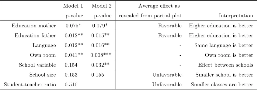
p-value p-value revealed from partial plot Interpretation Education mother 0.075* 0.079* Favorable Higher education is better Education father 0.012** 0.015** Favorable Higher education is better Language 0.012** 0.016** - Same language is better Own room 0.041** 0.008*** - Own room is better School variable 0.154 0.032** - E¤ect between schools School size 0.153 0.155 Unfavorable Smaller school is better Student-teacher ratio 0.510 Unfavorable Smaller classes are better

where "***" denotes signi…cance at 1% level, "**" at 5% and "*" at 10%.

line with the general (parametric) literature (see Sirin (2005) for a comprehensive overview of published articles between 1990 and 2000):

- More educated parents will stimulate and encourage their children, such that for a given study devotion these will obtain higher test results.

- Children which are facing language di¢culties at school (because they speak a di¤erent language at home) obtain for a given e¤ort lower test results.

- Besides creating a good study environment, the possession of an own room can proxy the wealth of the family. Pupils with an own room (or, alternatively, from a wealthier family) obtain better results.

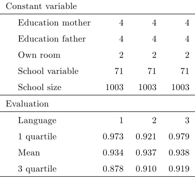
Table 6: Evaluation of general exogenous variables - example for native language

Constant variable

Education mother 4 4 4 Education father 4 4 4

Own room 2 2 2

School variable 71 71 71 School size 1003 1003 1003 Evaluation

Language 1 2 3

1 quartile 0.973 0.921 0.979 Mean 0.934 0.937 0.938 3 quartile 0.878 0.910 0.919

Finally, as mentioned above we can use partial regression plots to visualize the e¤ect of the exogenous environment. In a generalized multivariate framework, we set all other exogenous variables on their median value and, respectively, on their …rst and third quartile value to capture the heterogeneity among pupils. (Discrete variables are evaluated once at each category and continuous variables at 50 evaluation points.) We next illustrate the approach for the native language and for the school size. While keeping all other exogenous variables at their median value (or respectively at their …rst and third quartile value), we evaluate the variable (in casu the language) at its di¤erent data points (i.e. factors between 1, representing other language than any national language, and 3 the native language is the same as the test language).

0.86 0.88 0.9 0.92 0.94 0.96 0.98 1

0 1 2 3 4

Language

C

ondi

ti

onal

/

U

nc

ondi

ti

onal

eff

ic

iency

mean 25 quantile 75 quantile

Figure 1: Nonparametric plot of language

0.91 0.92 0.93 0.94 0.95 0.96 0.97 0.98 0.99 1 1.01

10 210 410 610 810 1010 1210 1410 1610

School size

C

ondition

al /

U

nc

onditio

nal ef

fic

ienc

y

25 quantile mean 75 quantile

6

Conclusion

This paper concentrates on conditional e¢ciency approach that accounts, in estimating rel-ative e¢ciency scores, for heterogeneity among the evaluated entities without assuming a separability condition (i.e. the environmental variables do not a¤ect the level of the in-puts and outin-puts). We explored the probabilitistic framework where conditional e¢ciency approach is relying on and argued that the traditional model faces two main drawbacks. Firstly, it has only been developed for continuous exogenous variables. In more interesting real life applications, the researcher wants to investigate the performance of entities while accounting for a broad set of exogenous variables, including both continuous and categorical (discrete) variables. By using insights from recent nonparametric econometrics literature we generalized the conditional e¢ciency model to mixed heterogeneous variables. Moreover, we proved that in our setting the discrete component does not su¤er from the curse of dimension-ality problem, which is the case for continuous environmental variables. Therefore, one can include a number of discrete environmental variables without reducing the accuracy of the estimation considerably. Secondly, apart from analyzing some descriptive …gures, no statisti-cal inference tools have been used in previous studies to test the signi…cance of the exogenous variables. Based on appropriate nonparametric econometric tests, we presented bootstrap procedures for testing the signi…cance of continuous and discrete environmental variables in the production process. In contrast to inference based on more traditional two-stage models, these tests can be used without assuming separability and without any parametric functional forms.

The suggested approach was illustrated using simulated examples as well as a sample of the OECD Pisa data set. In the empirical application, we examined the performance of British secondary school pupils while taking into account a broad range of continuous, or-dered as well as unoror-dered discrete exogenous factors. We …nd a signi…cant impact on the educational process for each of the discrete exogenous variables included in the application. This illustrates that in conditional e¢ciency estimation one should not limit only to continu-ous environmental variables, but also control for the heterogeneity resulting from the ordered and unordered discrete exogenous factors.

References