R&D, innovation and productivity, and the CIS: sampling, specification and comparability issues

RD, innovation and productivity, and the

CIS: sampling, specification and

comparability issues

Criscuolo, Chiara and Mariagrazia, Squicciarini and Olavi,

Lehtoranta

2010

Online at

https://mpra.ub.uni-muenchen.de/39261/

File name:  Criscuolo_Squicciarini_Lehtoranta_Concord2010.doc 

Author:  Mariagrazia Squicciarini 

Authors' contact:  mariagrazia.squicciarini@vtt.fi 

Status:  Draft 

Last updated:  21 Dec 2009 

Organisation:  VTT Technical Research Centre of Finland 

Knowledge for Growth – Industrial Research & Innovation (IRI)

R&D, Innovation and

Productivity, and the CIS:

Sampling, Specification and

Comparability Issues

Authors  Chiara Criscuolo 1 _{, Mariagrazia Squicciarini} 2 _{, Olavi Lehtoranta} 2 

1) _{London School of Economics, Centre for Economic Performance}  2) _{VTT Technical Research Centre of Finland, Innovation Studies}

Contributed paper for the 2

_{Conference on corporate R&D}

(CONCORD - 2010)

CORPORATE R&D: AN ENGINE FOR GROWTH,

A CHALLENGE FOR EUROPEAN POLICY

Abstract

We construct and estimate a modified version of the Crépon, Duguet and Mairesse (1998)  model to investigate the links between R&D, innovation output and productivity. We propose a  model specification that, among other features, aims to better capture the variance component  of the cooperation and obstacles­to­innovation variables. Results based on Finnish CIS data 

support this alternative specification and highlight the role of process innovations. We also  address comparability over time within the same country, by comparing Finnish CIS3 and  CIS4 estimates. Despite CIS harmonization, both sample selection issues and nuances in the 

specification of the variables prove to have a profound effect on the results, and question the  validity of this currently popular comparison exercises.

TABLE OF CONTENTS

1 ­  Introduction ...4 

2 ­  The Data ...4 

2.1  Sampling and data issues...4 

2.2  Descriptive statistics...6 

3 ­  Econometric model and variables used ...9 

3.1  The CDM model and its successors...9 

3.2  Main features of our model...10 

3.2.1  The estimation strategy ...10 

3.2.2  Model specification and definition of the variables ...11 

4 ­  Estimates and results...14 

5 ­  Conclusions and policy implications...17 

6 ­  Acknowledgments ...18 

1 ­ 

Introduction

Research and development (R&D) activities are believed to serve two main purposes. They  enhance absorptive capacity (Cohen and Levinthal, 1989), thereby facilitating the imitation of  others’ discoveries (Griffith, Redding and Van Reenen, 2004) and the absorption of new  technologies (Parisi, Schiantarelli and Sembenelli, 2006), and stimulate innovation. This  indirectly affects productivity, as innovation effort significantly determines innovation output,  and higher innovation output generally correlates positively with productivity (Crépon, Duguet  and Mairesse, 1998; Griffith et al., 2006). 

Since the pioneering work of Mansfield (1972) and Griliches (1979, 1992, 1998), the  relationship between R&D, innovation output and productivity has been the focus of many  microeconometric studies. Examples of early works are Odagiri (1984), Odagiri and Iwata  (1986), Chakrabarti (1990), and Hall and Mairesse (1995). More recently, studies mainly  exploiting data from the Community Innovation Survey (CIS) have contributed to verify the  existence of, and to quantify, the link R&D investment ­ innovation output – productivity, to  inform innovation policy. A large number of these studies rely on variants of the model first  proposed by Crépon, Duguet and Mairesse (henceforth CDM) in 1998, including, among  others, Lööf and Heshmati (2002), Griffith et al. (2006), Chudnovsky, López and Pupato  (2006), and the OECD (2009). 

The present paper contributes to this literature by addressing and providing empirical evidence  on three features of CIS data­based CDM­type models. Firstly, we investigate whether and to  what extent differences in the sampling frames within the same country, across different CIS  waves, affect the estimates. Secondly, we investigate whether the use of variables aimed to  exploit the richness of the information available in the CIS related to firms’ cooperation and  obstacles to innovation improves the fit of the model we propose. We find that it does improve  the overall fit of the model, and that the estimates shed light on the type of hindering factors  and collaborations that can affect R&D and innovation. Thirdly, by comparing Finnish CIS3  and CIS4 estimates, we verify the suitability of the new specification proposed and the  robustness of the model. 

The paper is organised as follows. Section 2 illustrates how the samples were constructed,  and provides some descriptive statistics relating to the data used in the study and their 

sources. Section 3 outlines the econometric model, its main features, and its main differences  with the original CDM model and variants of the CDM model in the literature. Section 4 

presents the estimates and discusses the results. Section 5 concludes with a summary of the  main findings of the analysis, and outlines possible implications for innovation policy. 

2 ­  The Data

2.1  Sampling and data issues

introduce, or is in the process of introducing, a new or substantially improved product or  process. 

CIS surveys are always retrospective in nature, in that they ask for information on the  innovative activities of firms in the previous three years. Only a portion of the information  collected is quantitative, whereas most data are collected in the form of the respondents’  subjective evaluation, expressed categorically on a Likert type scale. 

In the case of Finland, CIS3 and CIS4 questionnaires are almost identical in terms of number  and types of questions, with the exception of minor differences in the way some questions are  formulated. Moreover, Finnish CIS3 and CIS4 questionnaires both contain “filter questions”,  i.e. questions that, if answered negatively – thus implying that the firm did not innovate during  the period considered – allow respondents to skip the majority of the remaining questionnaire.  This ultimately means that very little information can be gleaned about non­innovators and  about their employment patterns, main industry, most important markets (e.g. domestic versus  foreign), and obstacles to innovation. Such a feature of the CIS somewhat impinges upon the  breadth and depth of the analysis that can be carried out. Information on non­innovators is in  fact of particular relevance for econometric analysis: the more information that is available on  non­innovators, the more precise will be the analysis of innovation determinants; and the  better the understanding of differences between innovating and non­innovating firms, i.e.  which firms are and which are not innovators. 

Despite being very similar in most aspects, Finnish CIS3 and CIS4 differ in with respect to  some important aspects. We highlight each in turn. 

A first and important difference in the CIS3 and CIS4 samples is that, in addition to the  stratified sample, CIS3 also includes a panel of firms known to be innovative on the basis of  CIS2 or CIS2.5. This feature of CIS3 may determine a selection bias, and questions the  representativeness of the sample. As innovative activities are persistent (Cefis, 2003), these  firms are more likely to be innovators than their randomly selected counterparts. 

A second major difference between the Finnish CIS3 and CIS4 concerns how the data have  been collected. CIS3 sampled firms were contacted via mail, whereas CIS4 firms received  both hard copy (surface mail) and e­questionnaire forms. 

A third main difference is that while response to CIS3 was voluntary, response to CIS4 was  mandatory. Response rates were 50% for CIS3 and 74% for CIS4. This substantial increase in  the CIS response rate (almost 50% more) can hence only partially – if at all – be attributed to  the way in which firms were contacted and given the possibility to respond. The major factor  driving the observed higher CIS4 response rate is most likely to be the fact that responding  was compulsory. This shift from voluntary to mandatory response was possibly intended to  minimise the possible self­selection biases characterising CIS respondents. As innovation is  generally held to be a “good thing”, innovative firms may have a greater incentive than non­  innovators to respond. This would ultimately result in innovators being over­represented in the  respondents’ samples, thus jeopardising the representativeness of CIS. 

contained in the Structural Business Statistics (SBS). Additional firm information has also been  gathered from the SBS. This is the case, for instance, of CIS4 data related to firms’ geographic  market reach, i.e. whether national or international. 

The presence of imputations and replacements, in addition to the other CIS features and  differences mentioned above, indeed represent an additional source of concern in the present  analysis, due to the biases they may introduce. Nevertheless, and despite the above 

considerations and concerns about the quality and reliability of CIS data, innovation surveys  remain unique and useful tools for attempting to answer important policy relevant questions.  We believe the gains that might be derived from relying on CIS data far outweigh the possible  drawbacks associated to their use, since they contain innovation­related information that  cannot be found anywhere else. Moreover, there is no such a thing as perfect data, and in the  case of CIS at least we know what to worry about, and may attempt to address possible  biases. 

2.2  Descriptive statistics 

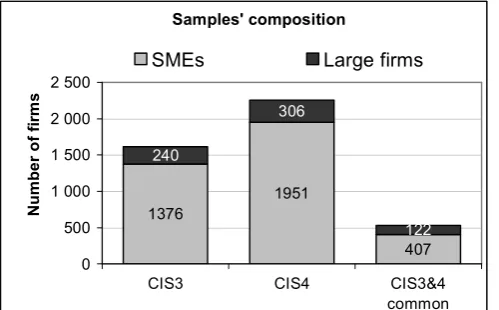
Figure 1 and Table 1 show the composition of CIS3 and CIS4 samples, in terms of Small and  Medium Sized Enterprises (SMEs) and large firms, as well as the composition of the sub­  sample of firms common to both CIS3 and CIS4. As can be seen, the total number of firms  varies enormously between the two CIS waves, but the share of SME and large firms differ  only marginally between the Finnish CIS3 and CIS4 samples. 

Figure 1: Sample composition  Table 1: Sample composition 

Source: Authors’ calculations using Statistics Finland data 

Table 2 shows the composition of CIS3 and CIS4 samples in terms of high­tech and low tech  manufacturing, and knowledge­intensive services sectors. Manufacturing, whether high­ or  low­tech, accounts for a bigger share of CIS3 firms compared to CIS4, whereas the opposite  is true for the service sector. 

1 _{Descriptive statistics are based on the unweighted samples and, therefore, do not correspond to the official}  statistical estimates for Finland. 

Samples’ composition in % 

SMEs  Large _firms  Tot # _firms 

CIS3  85.1  14.9  1616  CIS4  86.4  13.6  2257  Common 

CIS3&4  76.9  23.1  529 

Samples' composition 

1376  1951 

407 

240 

306 

122 

0  500  1 000  1 500  2 000  2 500 

CIS3  CIS4  CIS3&4  common 

Num

be

r o

f fi

rm

s

Table 2: Sample composition: percentage of high and low tech firms, and knowledge  intensive services 2 

CIS3 and CIS4 full samples  Common CIS3&4 sample 

SMEs  Large firms  Total 

Sector  CIS3  CIS4  CIS3  CIS4  CIS3  CIS4  SMEs  Large firms  Total 

High­tech manufacturing  18.4  16.5  4.3  3.0  22.6  19.5  21.8  6.6  28.4  Low­tech manufacturing  36.4  32.1  5.6  5.0  42.0  37.1  37.9  10.4  48.3  Knowledge intensive services  14.9  16.0  1.9  2.1  16.8  18.1  9.3  1.9  11.2  Other services  15.5  21.8  3.0  3.5  18.6  25.3  8.0  4.2  12.1 

Total  85.1  86.4  14.9  13.6  100  100  76.9  23.1  100 

Source: Authors’ calculations using Statistics Finland data 

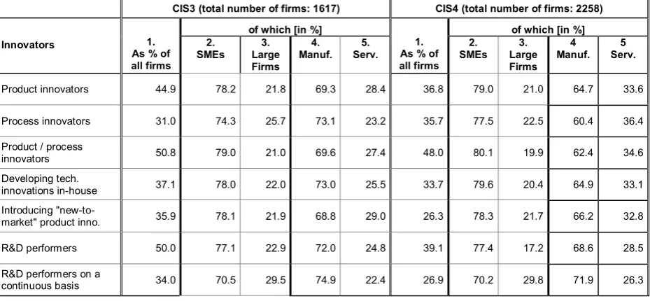
As for firms’ innovation patterns, Table 3 shows, for both CIS3 and CIS4, the percentage of  firms: innovating over the period considered; introducing product and process innovations;  developing technological innovations in­house; introducing "new­to­the­market" product  innovations; investing in R&D over the period considered; investing in R&D on a continuous  basis. Column 1 shows the percentage of the total number of firms. Columns 2 and 3  respectively, highlight how SMEs and large firms contribute to the overall share, while  columns 4 and 5 indicate how the share in column 1 is subdivided between manufacturing  and service sectors firms. 

We can see that the share of innovating firms ­ whether in processes or products ­ decreases  slightly (­2.8%) 3 _{from CIS3 to CIS4, and that a much lower share of CIS4 respondents (­9.6%)} 

has introduced “new­to­the­market” products than in CIS3. We also see that, compared to  CIS3, CIS4 firms seem less keen on developing technological innovations in­house, and that  the share of R&D performers decreases substantially: 50% in CIS3 versus 39.1% in CIS4. 

Table 3: CIS3 and CIS4: Innovation patterns, by firms size and industry 

CIS3 (total number of firms: 1617)  CIS4 (total number of firms: 2258) 

of which [in %]  of which [in %] 

Innovators  1. 

As % of  all firms 

2. 

SMEs  Large 3. 

Firms  4. 

Manuf.  Serv. 5.  As % of 1.  all firms 

2. 

SMEs  Large 3. 

Firms  4 

Manuf.  Serv.5   

Product innovators  44.9  78.2  21.8  69.3  28.4  36.8  79.0  21.0  64.7  33.6 

Process innovators  31.0  74.3  25.7  73.1  23.2  35.7  77.5  22.5  60.4  36.4 

Product / process 

innovators  50.8  79.0  21.0  69.6  27.4  48.0  80.1  19.9  62.4  34.6  Developing tech. 

innovations in­house  37.1  78.0  22.0  73.0  25.5  33.7  79.6  20.4  64.9  33.1  Introducing "new­to­ 

market" product inno.  35.9  78.1  21.9  68.8  29.0  26.3  78.3  21.7  66.2  32.8 

R&D performers  50.0  77.1  22.9  72.0  24.8  39.1  77.4  17.2  68.6  28.5 

R&D performers on a 

continuous basis  34.0  70.5  29.5  74.9  22.4  26.9  70.2  29.8  71.9  26.3 

Source: Authors’ calculations using Statistics Finland data 

Two additional features emerge when comparing CIS3 and CIS4 innovators’ figures. Firstly,  the proportions of innovators, in terms of SME and large firms, remain basically the same  across the various categories. Secondly, there are big differences in terms of the contributions  of the manufacturing and service sectors, with the latter playing a more important role in CIS4  than in CIS3. 

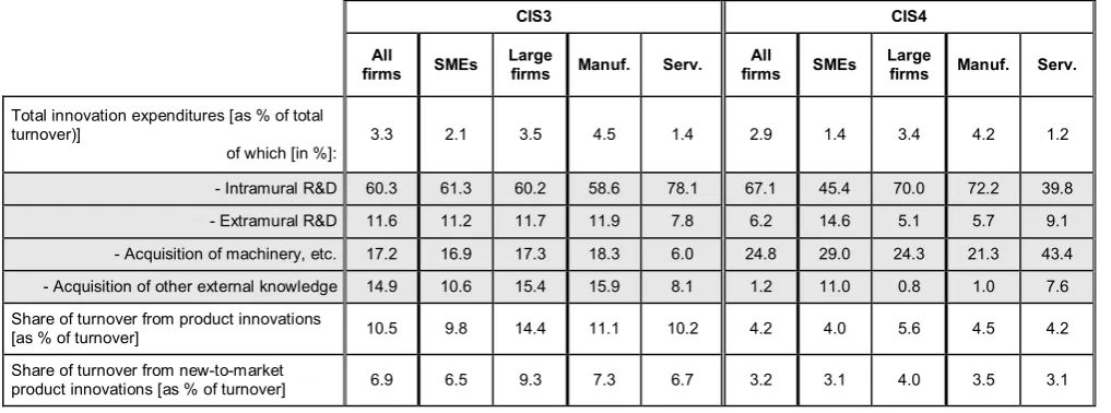
Table 4 shows firms’ innovation expenditure as share of total turnover, and its composition in  terms of intramural versus extramural R&D spending, as well as acquisition of machinery and  equipment and of external knowledge. 

Table 4: CIS3 and CIS4 Innovation expenditures and turnover from innovation, by firm  size and industry 

CIS3  CIS4 

All 

firms  SMEs  Large firms  Manuf.  Serv.  firms All  SMEs  Large firms  Manuf.  Serv. 

Total innovation expenditures [as % of total  turnover)] 

of which [in %]:  3.3  2.1  3.5  4.5  1.4  2.9  1.4  3.4  4.2  1.2  ­ Intramural R&D  60.3  61.3  60.2  58.6  78.1  67.1  45.4  70.0  72.2  39.8  ­ Extramural R&D  11.6  11.2  11.7  11.9  7.8  6.2  14.6  5.1  5.7  9.1  ­ Acquisition of machinery, etc.  17.2  16.9  17.3  18.3  6.0  24.8  29.0  24.3  21.3  43.4  ­ Acquisition of other external knowledge  14.9  10.6  15.4  15.9  8.1  1.2  11.0  0.8  1.0  7.6  Share of turnover from product innovations 

[as % of turnover]  10.5  9.8  14.4  11.1  10.2  4.2  4.0  5.6  4.5  4.2  Share of turnover from new­to­market 

product innovations [as % of turnover]  6.9  6.5  9.3  7.3  6.7  3.2  3.1  4.0  3.5  3.1 

Source: Authors’ calculations using Statistics Finland data 

The lower percentage of total innovation expenditures observed in the case of CIS4 (­0.4%)  seems mostly due to SME and the manufacturing sector investing less than in the CIS3  period. We can also see that, overall, CIS4 firms appear to be more inward looking than their  CIS3 counterparts, when it comes to investing in R&D, and to be less keen on outsourcing  R&D or acquiring external knowledge. The opposite is true for the acquisition of machinery  and equipment, where expenditure increases substantially in CIS4. 

With respect to the innovation­related output, a striking feature emerges: the share of turnover  generated from product innovations plunges from 10.5% in CIS3 to 4.2% in CIS4. The results  are similar for the introduction of products claimed by firms to be new to the market. 

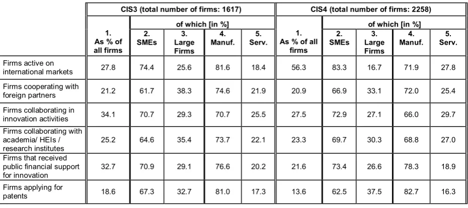
About firms’ degree of internationalisation, Table 5 4 _{suggests CIS4 respondents to be indeed} 

Table 5: Firms’ collaboration, financial support, degree of internationalization, and patenting 

CIS3 (total number of firms: 1617)  CIS4 (total number of firms: 2258) 

of which [in %]  of which [in %] 

1.  As % of  all firms 

2. 

SMEs  Large 3. 

Firms  4. 

Manuf.  Serv. 5.  As % of all 1.  firms 

2. 

SMEs  Large 3. 

Firms  4. 

Manuf.  Serv.5.   

Firms active on 

international markets  27.8  74.4  25.6  81.6  18.4  56.3  83.3  16.7  71.9  27.8  Firms cooperating with 

foreign partners  21.2  61.7  38.3  74.6  21.9  20.9  66.9  33.1  72.0  25.4  Firms collaborating in 

innovation activities  34.1  70.7  29.3  70.7  25.5  27.5  72.9  27.1  66.0  29.7  Firms collaborating with 

academia/ HEIs / 

research institutes  25.2  64.6  35.4  73.7  22.1  23.3  69.7  30.3  68.8  27.0  Firms that received 

public financial support 

for innovation  32.7  70.9  29.1  76.6  20.2  21.6  73.4  26.6  78.3  18.9  Firms applying for 

patents  18.6  67.3  32.7  81.0  17.3  13.6  62.5  37.5  82.7  16.3 

Source: Authors’ calculations using Statistics Finland data 

CIS4 respondents are generally much less likely to have formal cooperation agreements for  innovation projects than their CIS3 counterparts (­6.6%), although the share of firms 

cooperating with High Education Institutions (HEIs) and research centres is fairly stable.  When we compare firms’ degree of cooperation and internationalisation across the two  surveys we find that CIS4 SMEs and the service sector are substantially more likely to  cooperate and to be internationalised. The only countertendencies relate to the use of  patents, which are generally decreasing from CIS3 to CIS4, both for SMEs and the service  sector. Finally, financial support for innovative activities is much more important in CIS4 than  CIS3, with 11.1% fewer firms receiving funding in years 2000­2002 ­ particularly SME and  (slightly so) the services sector. 

3 ­  Econometric model and variables used

3.1  The CDM model and its successors

Since the seminal paper of Griliches and Pakes (1984), full structural models have been used  to address the relationship between innovation input, innovation output and productivity, using  direct measures of innovative output obtained from innovation surveys. The underlying crucial  assumption, first made in the CDM model, is that innovation inputs determine innovation  outputs, and that innovation output in turn affects productivity. 

In the CDM model the link between R&D, innovation output and labour productivity is  formalised as a system of simultaneous equations. The structure of the model is recursive,  and is estimated based on French CIS1 data using Asymptotic Least Squares (ALS). The first  two equations describe the R&D investment decision. Firms decide whether and how much to  invest in R&D: only if the net returns on this investment (which are not observable by the  econometrician, but which are known to the firm) are positive, will firms actually record positive  R&D expenditures. As it is restricted to successful innovators, this relationship is estimated  using a generalised Tobit specification. The third equation is a knowledge production function, 

which has two versions in the CDM model: in one innovation output is measured by the  proportion of sales due to new and improved products; in the second innovation output is  measured by patents. The fourth equation is an augmented Cobb­Douglas value­added  production function. The latter two steps in the model are estimated for “innovative” firms only,  i.e. firms that spend on R&D. 

The CDM model corrects for two main problems normally affecting this type of analysis:  selectivity and endogeneity. Selectivity means that only a subset of firms invests in R&D.  Therefore, when the analysis is restricted to this non­random subset of “R&D spenders”, it is  necessary to correct for possible selection biases. Endogeneity implies that some of the  explanatory variables and the dependent variables might be simultaneously determined in the  model. For example, innovation inputs might be endogenous in the knowledge production  function, because firms that are more likely to innovate successfully (in terms of output) might  also be those that spend more on innovation. Likewise, innovation output might be 

endogenous in the output production function, either because of unobserved shocks, 

correlated with both total sales and the firm’s innovative sales, or because of unobserved firm  characteristics (e.g. management quality). 

Janz, Lööf and Peters (2004) estimate a variant of the CDM model on pooled firm level data  from the CIS3 of Sweden and Germany. This allows them to test for the equality of the model  parameters across these two countries. As in the CDM model, the estimates rely on innovative  firms only, but, rather than using just R&D expenditure, they use all innovation related 

expenditures as inputs in the knowledge production function. While allowing for possible  feedback effects of productivity on innovation output, Janz, Lööf and Peters do not assume a  fully recursive model. 

Griffith, Huergo, Mairesse and Peters (2006) apply another variant of the CDM model to data  from CIS3 (1998­2000) for France, Germany, Spain and the UK. In contrast to CDM, they  estimate the model on all firms in the manufacturing sector, as they believe that firms reporting  zero R&D may still have positive knowledge outputs. The underlying assumption here is that  the relationship between innovation inputs and innovation outputs is the same for firms that  report positive R&D and firms that report zero R&D. The model is estimated separately for  each country and, therefore, coefficients are allowed to vary across countries, and their  equality across countries cannot be tested. 

The OECD Innovation Microdata Project (2009) – in which the authors participated – includes  a cross­country CDM­type analysis based on data from CIS4 for the EU  countries and data  for New Zealand, Australia, Canada, Korea and Brazil, where innovation surveys are 

formulated in a similar but not fully harmonized way. This very broad geographical coverage  has some drawbacks in terms of the richness of the final specification of the model, because it  constrains the regressors and controls that can be used. In fact, the variables included in the  model constitute a minimum, common denominator set of variables chosen in order that the  same model can be applied to all countries.  Moreover, due to confidentiality issues, the data  were not pooled, thus making it impossible to test the equality of the model coefficients across  participating countries. 

3.2  Main features of our model

3.2.1  The estimation strategy

firms that conduct their innovative activities more informally could in fact register zero R&D  expenditures, but still invest in innovation. In the second step we estimate the model only for  innovative firms, defined as firms with positive innovation expenditure and positive innovative  sales, and not on all firms, as Griffith et al. (2006) instead do. We are motivated by the belief  that holding the underlying relationship between innovation input and output to be the same for  all firms, whether innovative or not, is too strong an assumption. 

Finally, and similarly to OECD (2009), the third step in our model estimates the elasticity of  productivity with respect to product innovation, but only for innovative firms. While 

acknowledging the importance of process innovation ­ which was absent from the original  CDM model, but included in Griffith et al.’s model ­ we do not to have a separate innovation  output equation for process innovations. We prefer to include process innovation as an  additional control, in both the product innovation function and the productivity equation, as we  believe that the two phenomena are highly interlinked. 

We estimate the innovation investment and innovation output equations simultaneously, using  a two step limited information maximum likelihood method.  Following CDM, we allow for the  endogeneity of both input and output of the innovation process, but –unlike Janz, Lööf and  Peters (2004) ­ we do not allow for potential feedback effects of productivity on innovation  output. Finally, to avoid the possible biases that may arise when using data coming from  different sources, as in the OECD model, we use only the variables available in the innovation  surveys. This choice, which is the same made by the OECD (2009), if on the one hand 

minimises the possible sources of bias, on the other hand leads us to using a very simple  productivity measure, namely the log of sales per employee. 

3.2.2  Model specification and definition of the variables

Similar to CDM, we use a three­stage four­equation model. The first stage explains the firm’s  decision to engage (or not) in innovation activities, and the amount of innovation expenditure  chosen. It comprises two equations and is estimated using a generalised Tobit model 

(Heckman, 1979). The first equation accounts for firms’ innovative efforts (innov*) and can be  formally written as follows: 

Innovi*=X’1ib+ui 

where subscript i indicates firms; X is a vector of regressors that we describe below and u is  the error term that we assume is normally distributed. As firms will innovate only if the net  gains from this activity are positive, we observe the discrete event of whether firm i  is 

innovative or not, rather than observing the latent variable Innov*. Therefore, the first equation  models the probability that the firm is innovative using a probit model: 

Prob(Innovi=1)=Pr(Innovi*>0)= Pr(ui >­X’1ib) 

X’1 is a vector of variables affecting the innovation investment decision and includes: size of 

the firm, measured as log employment (“LEMP”); a dummy for whether the firm is part of a  group or not (“GROUP”); a dummy for whether the firm serves foreign markets or not  (“FOR_MKT”), as well as industry dummies. The X’1 vector also includes a set of variables 

used to capture the intensity of the obstacles firms may face when innovating. These are  knowledge, costs and market­related obstacles. Unlike the OECD model, the obstacle related  variables are specified here as variables taking values between 0 and 1. “HACOST” accounts  for the intensity of cost­related obstacles; “HAKNOW” for intensity of knowledge­related 

3, depending on whether the problem is rated respectively “low”, “medium”, or “high”. Zero  values are attributed in the case a firm declares not to have experienced the problem. The  figures thus obtained for each problem­related question are added together, to produce a  figure in the zero to 9 range (i.e. three questions, each with values from zero to 3). This figure  is then divided by 9, i.e. the maximum possible value, to normalise the variable. Lastly, a  variable called “OBS” constructed as: OBS = (“HACOST”+ “HAKNOW”+“HAMARKET”)/3  summarises the overall intensity of all the obstacles. The choice of the covariates used in this  equation is mainly dictated by the limited availability of information for non­innovative firms.  Conditional on the firm being innovative, we observe a firm’s innovation investment intensity to  be: 

InnExp= X’2 d + ei  if  Innov=1  and 

InnExp= 0  if  Innov=0 

The second equation in the first stage is an innovation expenditure equation, where the 

dependent variable is innovation expenditure per employee. The equation estimates the role of  exogenous covariates on the amount of innovation expenditure. We assume the error terms u  and e to be jointly normally distributed, with mean zero and covariance rho, and estimate the  two equations as a generalized Tobit equation, by maximum likelihood. 

Relative to the first equation, we use additional regressors. In particular, we include a dummy  accounting for whether the firm cooperates or not (“COOP”) and a set of four variables 

accounting for the various types of cooperation, their intensity and their geographical reach.  The dummy “COOP” takes the value 1 if firms have any kind of collaboration whatsoever, i.e. if  they answered yes to at least one of the collaboration­related questions. “COOP_own_chain”  takes positive values 5 _{if the firm responds as cooperating internally (i.e. with other} 

branches/units of the same enterprise), and/or with suppliers and clients, and zero otherwise.  Similarly, the variable “COOP_out_private”, accounts for the firm’s collaboration in innovative  activities with competitors and consultants. Finally “COOP_out_public” captures the firm’s  degree of collaboration with HEIs and universities, as well as research centres. 6 The 

cooperation­related variables are constructed in such a way as to capture whether the firms is  inward­looking – i.e. it mainly relies on its “own chain” when innovating, or outward looking ­  implying that it seeks the support of external partners, both private and public institutions. In  addition, the variable “COOP_intern” accounts for the degree of internationalisation in firms’  collaborations. It is constructed as a ratio in which the numerator is the number of international  collaboration­related items that firms ticked in the questionnaire, and the denominator is the  numerator plus the number of all national collaboration­related items ticked. 7 

A crucial assumption in identifying the parameters of interest is the existence of exclusion  restrictions, i.e. variables affecting the decision to invest in innovation, but not the intensity of  the innovation effort. Our exclusion restrictions are firm size and obstacles to innovation. The  idea is that, while it is well known (Schumpeter, 1942; Cohen and Klepper 1992; and Klette  and Kortum, 2004) that larger firms are more likely to invest in innovation, innovation 

investment intensity ­ measured as the ratio of total innovation expenditure per employee ­ is  already scaled and therefore less likely to be correlated to size. 8 _{Moreover, we believe that the} 

obstacles to innovation that firms may encounter would condition their decisions about  whether or not to innovate, but not about how much to invest in innovation. 

5 _{Between 1 and 12. Firms were given the possibility to tick all 12 boxes related to the specific type of cooperation}  considered. In turn, each type of collaboration, i.e. within own firm, with suppliers, and with clients, was subdivided  into 4 regions, depending upon the geographic level of the collaboration: national, within Europe, with the USA,  with the rest of the world. 

6 _{“COOP_out_private” and “COOP_out_public” values range between 0 and 18, as they are based on two}  questions each and are related to four regions, as in the case of “COOP_own_chain”. 

7 _{If none of these boxes were ticked, the variable takes zero value.} 

Finally, from this first step we estimated the inverse Mills ratio, to be used as an additional  regressor in the second and third steps of the model, to control for selectivity. Also, we predict  innovation expenditure. 

In the second step of the model, we estimate a knowledge production function where the  dependent variable, log innovative sales per employee, depends on: the intensity of  investment in innovation (“LISPE”); firm size; whether or not the firm is part of a group; a  dummy accounting for whether or not the firm has carried out process innovation 

(“PROCESS”); the cooperation variables, as described above; the industry dummies, and  dummies for the obstacles to innovation­related regressors. Since we estimate the model for  innovative firms only, we include the Mills ratio estimated in the first stage to correct for 

selectivity. We also present the results where, in addition to selectivity, we control for potential  endogeneity of innovation expenditure in the knowledge production function. Endogeneity  might arise because of unobserved heterogeneity or because of omitted variables, i.e. factors  that we do not control for but that can influence firms’ innovation output and are likely to affect  innovation inputs (e.g. positive temporary shocks; unobserved managerial ability, etc.). 

Endogeneity might also arise because of “simultaneity”, as the innovation surveys ask for  innovation inputs and outputs related to the same years. The way we chose to proceed is to  use predicted rather than actual innovation expenditure in the knowledge production function.  The identification restriction here is that public financial support only affects innovation 

outcome through increased innovation investment and, similarly, that – once we condition for  the cooperation activity of the firm – serving foreign markets only affects innovation output  through increased innovation expenditure. 9 _{Formally, the innovation outcome equation can be} 

written as: 

Innov_output= X’3 g + vi 

Innov_output is measured as log innovative sales per employee and the vector of covariates  X’3 contains the variables mentioned above, plus the actual log innovation expenditure per 

employee (“LRTOTPE”). When correcting for potential endogeneity, we use predicted values.  In the third and last stage of the model we estimate the innovation output productivity link  using an augmented Cobb­Douglas production function. 

Ln(sales per employee)= X’4 p + vi 

The dependent variable is log sales per employee (“LLPPE”). The right hand side variables  include: firm size; the group dummy, the innovation process dummy; the Mills ratio to correct  for selectivity; and log innovative sales per employee. The output production function is  estimated using Instrumental Variables 2­Stage Least Squares (IV 2SLS), to account for the  potential endogeneity of log innovative sales per employee. 

Since in the last two stages of the model we use predicted values (Mills ratio and predicted  innovation input), we need to correct for standard errors and account for this feature in the  model. We do so by bootstrapping standard errors in the innovation and the output production  functions. 10 

9 _{The latter is a very strong assumption since we are not allowing international technology transfer to have any}  other potential roles than those resulting from formal cooperation agreements. 

4 ­  Estimates and results

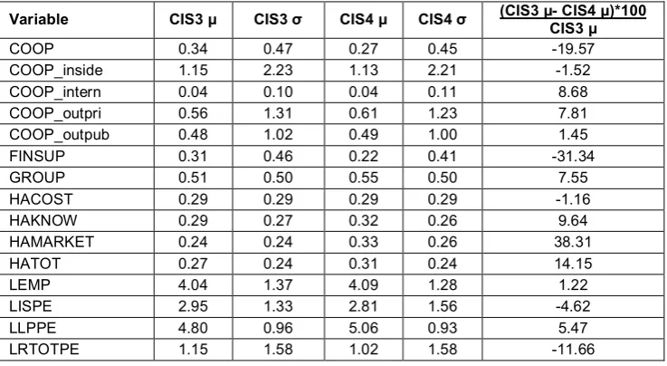
Here, we estimate the model described above, separately for the Finnish CIS3 and CIS4 data.  The aim is to verify the link between R&D, innovation output and productivity, and also to see  how results differ within the same country, depending upon how the samples have been built.  Before presenting the estimates and discussing the results, we provide two more tables  (Tables 6 and 7) showing the means and standard deviations of the variables used in the  model for CIS3 and CIS4, and for the sample of firms common to both. These figures are  meant to make some of the features discussed in section 2.1 numerically explicit, and will help  the interpretation and discussion of the estimates shown in Table 8. 

Table 6: Mean values and standard deviations of CIS3 and CIS4 variables 

Variable  CIS3 μ  CIS3 σ  CIS4 μ  CIS4 σ  (CIS3 μ­ CIS4 μ)*100 _CIS3 μ 

COOP  0.34  0.47  0.27  0.45  ­19.57 

COOP_inside  1.15  2.23  1.13  2.21  ­1.52 

COOP_intern  0.04  0.10  0.04  0.11  8.68 

COOP_outpri  0.56  1.31  0.61  1.23  7.81 

COOP_outpub  0.48  1.02  0.49  1.00  1.45 

FINSUP  0.31  0.46  0.22  0.41  ­31.34 

GROUP  0.51  0.50  0.55  0.50  7.55 

HACOST  0.29  0.29  0.29  0.29  ­1.16 

HAKNOW  0.29  0.27  0.32  0.26  9.64 

HAMARKET  0.24  0.24  0.33  0.26  38.31 

HATOT  0.27  0.24  0.31  0.24  14.15 

LEMP  4.04  1.37  4.09  1.28  1.22 

LISPE  2.95  1.33  2.81  1.56  ­4.62 

LLPPE  4.80  0.96  5.06  0.93  5.47 

LRTOTPE  1.15  1.58  1.02  1.58  ­11.66 

Source: Authors’ calculations using Statistics Finland data 

Table 7: Mean values and standard deviations of CIS3 & CIS4 common sample variables 

Variable  CIS3 μ  CIS3 σ  CIS4 μ  CIS4 σ  (CIS3 μ­ CIS4 μ)*100 _CIS3 μ 

COOP  0.41  0.49  0.37  0.48  ­8.51 

COOP_inside  1.54  2.54  1.75  2.74  13.63 

COOP_intern  0.05  0.12  0.06  0.12  21.26 

COOP_outpri  0.74  1.53  0.89  1.46  21.36 

COOP_outpub  0.61  1.14  0.76  1.25  23.15 

FINSUP  0.39  0.49  0.31  0.46  ­20.54 

GROUP  0.62  0.49  0.66  0.47  7.77 

HACOST  0.28  0.28  0.32  0.28  13.23 

HAKNOW  0.30  0.26  0.36  0.25  21.25 

HAMARKET  0.23  0.23  0.39  0.25  66.67 

HATOT  0.27  0.22  0.35  0.22  31.48 

LEMP  4.69  1.29  4.69  1.33  ­0.05 

LISPE  2.97  1.30  2.96  1.44  ­0.45 

LLPPE  4.91  0.88  5.11  0.82  4.00 

LRTOTPE  1.13  1.51  1.00  1.52  ­11.55 

Table 6 shows substantial changes between the values of the CIS3 and CIS4 variables related  to: overall cooperation (COOP), financial support (FINSUP), total obstacles encountered  (HATOT), market obstacles (HAMARKET), and R&D expenditures (LRTOTPE). In particular,  the differences for HAMARKET’s and FINSUP are higher than 30%, compared to the 

differences among the other variables, which range between 10% and 20%. 

Table 8 presents the estimates of our model for the CIS3 and CIS4 samples. 

With respect to the Heckman selection equation, i.e. the equation modelling the decision about  whether or not to invest in innovation, we see that being present in foreign markets and being  bigger in terms of number of employees correlates significantly and positively with investment  in innovation. The hampering factors firms may encounter when deciding to innovate also  positively and generally significantly correlate with the decision to innovate. This result is  somewhat counter­intuitive, as one would expect the obstacle­related variables to be  significant, but to exhibit negative coefficients. However, we believe these results might be  mirroring a sort of “ex­post rationalisation” by the innovators. In other words, it might be that  those firms putting effort into and managing to solve the innovation­related problems 

encountered might also be those that documented the existence of these problems, thus  making the coefficients significant and positive. 

From the innovation input equation – modelling the decision related to the size of the R&D  investment ­ it emerges clearly that there is a significant and positive correlation between the  intensive margin of the R&D investment and the fact that firms cooperate (COOP) and obtain  financial support (FINSUP). Conversely, the non significance of the GROUP­related 

R&D, Innovation and Productivity, and the CIS

(1)  (2)  (3)  (4)  (5)  (6)  (7)  (8)  (1)  (2)  (3)  (4)  (5)  (6)  (7)  (8) 

COEFFICIENT  Heckman _Outcome  Heckman _Selection  Producti. _(LLPPE)  Inno outcome 

(LISPE) 

ivLLPPE 

_hat  LISPE _hat  bstrap _llppe  bstrap _lispe  Heckman Outcome  Heckman Selection  Producti. (LLPPE) 

Inno  outcome  (LISPE) 

ivLLPPE 

_hat  LISPE _hat  bstrap _llppe  bstrap _lispe 

GROUP  ­0.120  0.00375  0.204***  0.224**  0.240***  0.230**  0.240***  0.230  0.184  0.0948  0.246***  0.223  0.237***  0.262*  0.237***  0.262 

(0.12)  (0.080)  (0.063)  (0.11)  (0.063)  (0.12)  (0.059)  (0.17)  (0.13)  (0.070)  (0.065)  (0.14)  (0.073)  (0.15)  (0.076)  (0.17) 

FOR_MKT  0.474***  0.260***  0.176  0.494*** 

(0.13)  (0.083)  (0.21)  (0.086) 

COOP  0.493***  0.481*** 

(0.12)  (0.12) 

FINSUP  0.703***  0.457*** 

(0.12)  (0.12) 

Sector dummies  yes  yes  yes  yes  yes  yes  yes  yes  yes  yes  yes  yes  yes  yes  yes  yes 

LEMP  0.227***  0.0884***  ­0.351***  0.0732**  ­0.515***  0.0732**  ­0.515***  0.247***  0.0962***  ­0.284***  0.0996***  ­0.328***  0.0996***  ­0.328*** 

(0.030)  (0.030)  (0.10)  (0.030)  (0.12)  (0.036)  (0.13)  (0.028)  (0.029)  (0.10)  (0.031)  (0.10)  (0.033)  (0.11) 

HACOST  0.283*  ­0.341  ­0.487**  ­0.487  0.0834  ­0.426*  ­0.381  ­0.381 

(0.16)  (0.23)  (0.24)  (0.36)  (0.13)  (0.23)  (0.24)  (0.26) 

HAKNOW  0.846***  ­0.880**  ­1.093**  ­1.093*  0.514***  ­0.0574  ­0.0439  ­0.0439 

(0.19)  (0.43)  (0.50)  (0.63)  (0.17)  (0.35)  (0.36)  (0.39) 

HAMARKET  0.114  ­0.644**  ­0.664**  ­0.664  0.687***  ­0.781**  ­0.780**  ­0.780* 

(0.21)  (0.30)  (0.31)  (0.45)  (0.17)  (0.37)  (0.38)  (0.47) 

LISPE  0.433***  0.339***  0.339***  0.329***  0.355***  0.355** 

(0.066)  (0.094)  (0.089)  (0.072)  (0.11)  (0.15) 

PROCESS  ­0.105*  0.332***  ­0.0600  0.362***  ­0.0600  0.362***  ­0.0688  0.274**  ­0.0780  0.304**  ­0.0780  0.304** 

(0.059)  (0.099)  (0.061)  (0.10)  (0.067)  (0.11)  (0.057)  (0.12)  (0.068)  (0.13)  (0.085)  (0.13) 

MILLSstrict  0.160  ­2.095***  0.105  ­2.627***  0.105  ­2.627***  0.201  ­1.129**  0.208  ­1.144**  0.208  ­1.144* 

(0.14)  (0.65)  (0.14)  (0.83)  (0.15)  (0.96)  (0.12)  (0.56)  (0.13)  (0.57)  (0.14)  (0.60) 

COOP_inside  0.0327  0.0576**  0.0576**  ­0.0322  ­0.0242  ­0.0242 

(0.027)  (0.029)  (0.027)  (0.037)  (0.038)  (0.041) 

COOP_outpri  0.0425  0.0581  0.0581  0.101  0.0976  0.0976 

(0.038)  (0.038)  (0.038)  (0.064)  (0.064)  (0.062) 

COOP_outpub  0.0339  0.109**  0.109*  ­0.0186  ­0.00184  ­0.00184 

(0.049)  (0.054)  (0.058)  (0.078)  (0.084)  (0.089) 

COOP_intern  ­0.500  ­0.358  ­0.358  0.872  1.351**  1.351* 

(0.49)  (0.49)  (0.52)  (0.64)  (0.62)  (0.69) 

­0.0555  ­0.0555  ­0.0151  ­0.0151 

LRTOTPE 

strict_hat  (0.13)  (0.15)  (0.23)  (0.30) 

Constant  ­0.354  ­1.639***  3.336***  6.381***  3.684***  7.873***  3.684***  7.873***  ­0.243  ­1.786***  3.634***  4.708***  3.556***  4.926***  3.556***  4.926*** 

(0.31)  (0.19)  (0.35)  (1.23)  (0.40)  (1.54)  (0.41)  (1.72)  (0.34)  (0.18)  (0.30)  (1.02)  (0.39)  (1.04)  (0.44)  (1.16) 

LRTOTPE  0.261***  0.198*** 

(0.036)  (0.043) 

Observations  1546  1546  688  688  688  688  1617  1617  2156  2156  699  699  699  699  2258  2258 

R­squared  .  .  0.42  0.27  0.45  0.20  0.45  0.20  .  .  0.36  0.14  0.34  0.11  0.34  0.11 

P­value LR test  0.00215  0.0680 

As for the other variables entering the innovation output equation, we see that the obstacles to  innovation generally (and significantly) impinge upon firms’ innovative output. In the CIS3  case, the hindering factor that seems to most severely disrupt innovative output is the lack of  the necessary knowledge, with HAKNOW coefficients in the range ­0.880 to ­1.093. 

Conversely, CIS4 innovators rate market­related difficulties to be the most severe hampering  factor to innovation, with a HAMARKET value of ­0.780. Another regressor entering the  innovation output equation that always turns out to be significant, and negative, is the  regressor for selection, i.e. the regressor related to the Inverse Mills ratio. MILLSstrict CIS3  values are generally more than double those in CIS4, suggesting that selectivity is a much  more important problem in CIS3 than in CIS4 (although in both cases selectivity is an issue).  While this result might be expected given the difference in the CIS3 and CIS4 sampling  procedures discussed in section 2.1, its robustness increases our concern about the way the  samples were constructed. 

Another feature common to both CIS3 and CIS4 estimates, is the positive and always  significant value of the variable for process innovations in the innovation output equation.  Hence, process innovations positively correlate to innovative sales, indirectly suggesting the  likely complementarity between process and product innovations. Results for the way that  different types of cooperation affect innovative sales are not clear­cut. In the case of CIS3, the  estimates seem to suggest that cooperating within the firm, and with public institutions, may  have a positive effect, whereas CIS4 estimates point to the positive role of cooperating at the  international level. Taken together, the coefficients of the obstacles­related variables and the  cooperation­linked regressors seem to suggest the following. In CIS3, firms perceive the lack  of the necessary knowledge to be most important factor hindering innovation. Collaborating  with universities and research centres seems to ease this lack of knowledge constraint, thus  positively affecting innovative output. For CIS4 firms, the most difficult problems seem to be  related to the markets targeted, especially international ones ­ and we know that the 

percentage of firms active in international markets jumped from 27.8% in CIS3 to 56.3 in CIS4.  Collaborating at the international level, therefore, may help firms to address and possibly solve  such problems, since we see that international collaborations significantly and positively relate  to innovative output. 

With respect to how R&D investments affect innovative output, we see that both CIS3 and  CIS4 estimates show significant and positive values of the R&D investment coefficient.  However, when using predicted values, the R&D coefficient is no longer significant. Hence,  further investigation is needed to check the robustness of our estimates to endogeneneity and  to the use of predicted values. 

Finally, concerning firm size, we see that being bigger is negatively correlated with innovation  sales, but positively correlated with productivity. In particular, the LEMP coefficients vary  between ­0.284 and ­0.515 in the innovation output equation, while the LEMP values in the  productivity equation range between 0.0732 and 0.0996. 

The last equation in our model, i.e. the productivity equation, suggests that firm size, belonging  to a group and innovative sales are all positively correlated to productivity. The coefficient of  the variable accounting for process innovation, on the other hand, has a negative sign, but  since it is basically never significant we cannot say that, in our model, process innovations  affect productivity. 

5 ­  Conclusions and policy implications

obtained. The third step mirrors the relationship between innovative output and productivity.  One important result from this model is that it captures the different characteristics of the CIS3  and CIS4 samples extremely well. In fact, both the signs and sizes of the coefficients generally  behave according to expectations and the estimates mirror the data features emerging from  the descriptive statistics. 

The estimates show that receiving financial support and having (relatively more intense)  collaborations are strongly and significantly correlated with a higher probability of engaging in  R&D activities. The amount invested in R&D is positively related to the size of the firm (in  terms of number of employees) and to the intensity of the obstacles faced. 

For innovative output, we see that investing in R&D is positively related to higher sales from  innovative goods. Another element that emerges is the positive relationship between product  and process innovations: process innovation seems to be complement product innovation and  is positively correlated to higher innovative sales. Conversely, we see that innovative output is  significantly and negatively affected by the problems firms may have encountered while  innovating. Both innovative output and productivity are shown to be positively related to  belonging to a group, and to firm size. Finally, and very importantly, innovative sales are  positively correlated to productivity. 

Our analysis supports the hypothesis of a positive link between investing in R&D, innovation  output and productivity, and has several interesting policy implications. Firstly, we observe a  positive correlation between the fact that firms collaborate and the size of their investments in  R&D. Secondly, we see that obtaining subsidies indeed eases firms’ budget constraint and  increases the likelihood that firms will invest in R&D. Nevertheless, firms still do encounter  problems in their innovative activities, and these are negatively correlated to sales from  innovative products. This latter result, coupled with the evidence that belonging to a group  correlates positively with both innovative sales and productivity, seems to suggest that 

innovating is difficult for firms, because of the cost, knowledge and market problems involved.  This seems to be especially true for individual firms, i.e. firms that do not belong to a group.  Hence, purposeful, well­formulated policies could ease the hampering factors firms encounter  by supporting their innovation activities from invention to the marketing of innovation. Policy  support should not stop once an innovation output is obtained; it needs to continue to enable  firms to transform innovative output into market success. 

Thirdly, our results suggest that product and process innovations are complementary. This  somewhar questions those policy programmes in which subsidies go preferably to those firms  whose innovative activities are expected to result in a product innovation (normally protected  by a patent). 

Finally, and with respect to the way that innovation data are gathered, there is a need to move  from CIS harmonisation to homogenisation of the way the samples are constructed and data  collected. This is especially true if the aim is to carry out cross­country comparisons, as  sample composition affects representativeness and comparability. In addition, simultaneity  problems – based on innovation input and output data referring to the same year – need to be  solved in order to better capture innovation dynamics. This can be done by collecting panel  data, i.e. by observing firms’ innovative behaviours over several years. 

6 ­  Acknowledgments

7 ­  References

Cefis E., Is there Persistence in Innovative Activities?, International Journal of Industrial  Organization 21 (4), 2003, pp. 489­515 

Chakrabarti A. K., Innovation and Productivity: An Analysis of the Chemical, Textiles and  Machine Tool Industries in the U.S., Research Policy, 19(3), 1990, pp. 257­269. 

Chudnovsky D., López A., Pupato G., Innovation and Productivity in Developing Countries: A  study of Argentine Manufacturing Firms' Behavior (1992­2001), Research Policy, Vol. 35(2),  2006, pp. 266­288 

Cohen W. M., Klepper S., The Anatomy of Industry R&D Intensity Distributions, American  Economic Review, Vol. 82(4), Sep., 1992, pp. 773­799 

Cohen W. M., Levinthal D.A., Innovation and Learning: The Two Faces of R & D, The  Economic Journal, Vol. 99(397), Sep. 1989, pp. 569­596 

Crépon B., Duguet E., Mairesse J., Research, Innovation and Productivity: an Econometric  Analysis at the Firm Level, NBER Working Paper 6696, Aug. 1998 

Dosi G., Sources, Procedures, and Microeconomic Effects of Innovation, Journal of Economic  Literature, Vol. 26(3), Sep. 1988, pp. 1120­1171 

Griffith R., Huergo E., Mairesse J., Peters B., Innovation and Productivity Across Four  European Countries, Oxford Review of Economic Policy, Vol. 22(4), 2006, pp. 483­498 

Griffith R., Redding S., Van Reenen J., Mapping the Two Faces of R&D: Productivity Growth  in a Panel of OECD Industries, Review of Economics and Statistics, Nov. 2004, No. 86(4), pp.  883­895 

Griliches Z., Issues in Assessing the Contribution of Research and Development to  Productivity Prowth, Bell Journal of Economics, Vol. 10(1), 1979, pp. 92 ­116. 

Griliches Z., The Search for R&D Spillovers, NBER Working Paper 3768, 1992 

Griliches Z., R&D and Productivity. The Econometric Evidence, The University of Chicago  Press, 1998 

Hall B. H., Mairesse J., Exploring the Relationship between R&D and Productivity in French  Manufacturing Firms, Journal of Econometrics, Vol. 65, 1995, pp. 263–293 

Hatzichronoglou T., Revision of the High­Technology Sector and Product Classification, OECD  Science, Technology and Industry Working Papers, 1997/2, 1997, OECD Publishing, 

doi:10.1787/134337307632 

Heckman J. J., Sample Selection Bias as a Specification Error, Econometrica, Vol. 47(1), Jan,  1979), pp. 153­161 

Janz N., Lööf H., Peters B., Innovation and Productivity in German and Swedish 

Manufacturing Firms: Is there a Common Story?, Problems & Perspectives in Management,  Vol. 2, 2004, pp. 184­204. 

Lööf H., Heshmati A., Knowledge Capital and Performance Heterogeneity: A Firm­Level  Innovation Study, International Journal of Production Economics, No. 76, 2002, pp. 61–85 

Mairesse J., Sassenou M., R&D Productivity: A Survey of Econometric Studies at the Firm  Level, NBER Working Paper No. W3666, Mar 1991 

Mansfield E., Contribution of R&D to Economic Growth in the United States, Science, Vol.  175(4021), Feb. 1972, pp. 477–486 

Odagiri H., Research Activity, Output Growth and Productivity Increase in Japanese  Manufacturing Industries, Research Policy, Vol. 14(3), 1985, pp. 117­130. 

Odagiri H., Iwata H., The Impact of R&D on Productivity Increase in Japanese Manufacturing  Companies, Research Policy, Vol. 15(1), 1986, pp. 13­19 

OECD, 2009. Innovation in Firms. A Microeconomic Perspective, OECD, Paris. 

Pakes A., Griliches Z., 1984. Estimating Distributed Lags in Short Panels with an Application  to the Specification of Depreciation Patterns and Capital Stock Constructs, Review of 

Economic Studies, Vol. 51(2), Apr. 1984, pp. 243­262 

Parisi M. L., Schiantarelli F., Sembenelli A., Productivity, Innovation and R&D: Micro Evidence  for Italy, European Economic Review, No. 50, 2006, pp. 2037–2061 

Schumpeter J. A., Capitalism, Socialism, and Democracy, Harper, New York, 1942