Optimal Path Finding Method Study Based on Stochastic Travel Time

(1)

Optimal Path Finding Method Study Based on Stochastic

Travel Time

Zhanquan Sun, Weidong Gu, Yanling Zhao, Chunmei Wang

Key Laboratory for Computer Network of Shandong Province, Shandong Computer Science Center, Jinan, China Email: [email protected]

Received July 22, 2013; revised August 25, 2013; accepted September 18, 2013

Copyright © 2013 Zhanquan Sun et al. This is an open access article distributed under the Creative Commons Attribution License, which permits unrestricted use, distribution, and reproduction in any medium, provided the original work is properly cited.

ABSTRACT

Finding optimal path in a given network is an important content of intelligent transportation information service. Static shortest path has been studied widely and many efficient searching methods have been developed, for example Dijkstra’s algorithm, Floyd-Warshall, Bellman-Ford, A*

et al. However, practical travel time is not a constant value but

a stochastic value. How to take full use of the stochastic character to find the shortest path is a significant problem. In this paper, GPS floating car is used to detect road section’s travel time. The probability distribution of travel time is estimated according to Bayes estimation method. The combined probability distribution of a feasible route is calculated according to probability operation. The objective function is to find the route that has the biggest probability to arrive for desired time thresholds. Improved Genetic Algorithm is used to calculate the optimal path. The efficiency of the proposed method is illustrated with a practical example.

Keywords: Optimum Path; Stochastic Travel Time; Genetic Algorithm; Floating Car

1. Introduction

Finding optimal paths in a given network is one of the most fundamental problems in network studies and has broad applications in the physical and social sciences and in engineering, particularly in the fields of computer science, operations research, and transportation engineering [1]. Static shortest path has been studied widely and many efficient searching methods have been developed, for example Dijkstra’s algorithm, Floyd-Warshall, Bell-man-Ford, A*

et al. Dijkstra’s algorithm is a graph search

algorithm that solves the single-source shortest path problem for a graph with non-negative edge path costs, producing a shortest path tree [2,3]. This algorithm is often used in routing as a subroutine in other graph algo-rithms. The Floyd-Warshall algorithm compares all pos-sible paths through the graph between each pair of verti-ces [4]. The Bellman-Ford algorithm is an algorithm that computes shortest paths from a single source vertex to all of the other vertices in a weighted digraph [5]. Bellman- Ford is based on the principle of relaxation, in which an approximation to the correct distance is gradually re- placed by more accurate values until eventually reaching the optimum solution. A*_{uses a best-first search and}

finds a least-cost path from a given initial node to one goal node [6,7]. It is an extension of Dijkstra’s algo-

rithm. Classical shortest path searching methods are based on fixed path costs. However, practical travel time of a road segment is a stochastic variable. Shortest path is a random variable also. Shortest path based on random travel time has been studied [8-10]. The studied methods are difficult to be used in practical because that the algorithms are difficult and the probability distribution of road section travel time is difficult to be obtained.

(2)

has been widely studied [13]. In this paper, norm distribution is considered.

After the travel time probability distribution being determined, how to find the optimal path based on stochastic distribution is a difficult problem. In the optimal path searching study, the least expected travel time is often taken as the objection [14]. In the optimum problem, it requires evaluating multiple integrals. Classic shortest path finding methods, such as Dijkstra’s algorithm, Floyd-Warshall, Bellman-Ford, A*_{and so on, are not}

suitable to be used here. Some heuristic methods have been adopted to resolve the optimal problem [15-17]. Based on previous research, GA-based routing algorithm has been found to be more scalable and insensitive to variations in network topologies. It is taken as the most efficient one. However, many paths generated through cross and mutation are unreasonable. For resolving the problem, some improved genetic algorithms were proposed. In this paper, the improved genetic algorithms proposed in [17] will be adopted to resolve the optimal path problem. At last, an example is analyzed to illustrate the efficiency of the proposed method.

2. Travel Time Distribution Estimation

Based on GPS Floating Car

2.1. Travel Time Calculation Based on GPS Floating Car

GPS floating car can provide localization data, speed, travel direction and time information. Data collection interval, which can be set according to practical requirement, is often set as 30 seconds. These data are the es- sential source for intelligent transportation systems. In a certain time interval, a road section maybe includes several sample points of a floating car. Travel speed of a road section can be calculated according to simple floating car. The calculation method is described as follows.

Let the length of a road section be denoted , the vehicle speed at the ith sample point be denoted by i and the number of sample point be denoted by . Let 0

denote the first sampling point, and 1 denote last sam-

pling point. Travel speed of the road section is calculated as follows. d p v t t





1

0 1 1

1 0 d ₁ 2 t t _p

t r r

r r

r

d d d

v t _v _v

d

v t t

t t t

 _          _  _ __    





 (1)

When the sample time interval is fixed, the formula can be simplified as

1 0 1 ₂ p p r r v v v v p    





(2)

d t

v

 (3)

2.2. Travel Time Distribution Estimation

A road section may include several floating cars in a sample time interval. The travel time of the road section based on each floating car can be calculated according to above introduced method. The probability distribution style is determined with hypothesis test method. The distribution parameters of travel time are determined with Bayes method. The estimation method is introduced as follows.

Suppose a continuous random variable be X ,

 

~ . , Θ

X f   , with continuous parameter space .

The parameter

Θ

’s priori density is 

 

. . MX is the observation space of X . Based on data points

1, , ,2 n

x x _ x , the Bayes’ theorem can be expressed as follows.







  



1 2

  

1 2

1 2 Θ

; , , ,

, , , Θ

; , , , d n n

n

l x x x

x x x

l x x x

           



   (4) where l



; , , ,x x1 2 xn



is the likelihood function of the observations.

When travel time of a road section obeys normal distribution, the probability distribution can be denoted by

 



2



2

1 exp

2 2

x

f x 

 

 _ 



 _

 _ _ (5)

Given n data points D0



x x1, , ,2  xn



, who obey a normal distribution, the two parameters’ joint priori-distribution according to Jeffrey’s method is





2

1 ,

   

 (6)

The expected values of the updated parameters  and

 are





1 2

ˆ d x x xn

D

n



_

_       (7)













0

2

2 2 1

0

2

2 2 1

0

ˆ d

1 _exp 1 _{d d} 2

1 _exp 1 _{d d} 2 n i n i n i n i D x x                             _ _       _ _     









 

(8)

According to above Bayesian method, the distribution of travel time can be determined.

3. Distribution of Shortest Path

(3)

vertices set, is the link set, and is the weight value set of . Let 1 2 k denote a path from start node to end node n. The travel time of sec-tion is denoted by i

E E 1

, 2,_

T

RS S _S S S

, 1 ,

i i k X that obey normal distribution N



 _i, _i



. The shortest path is denoted by variable . It can be calculated according to the fol-lowing equation.

Y

1 2

y x x _x_n (9) The travel time of each road section is supposed independent. According to probability theory, the sum of independent normally distributed variables is also normally distributed. The distribution parameters are as follows.

 









 n





 

1 2

1 2 n

X X X

X E X

            

 

1 2 1 2

2 2 2

1 2 n

X X

D X D X

             



n E X  n  X 

E Y E

E   D



(10)

 

D Y

 



n D X

 (11)

The distribution of shortest path y can be described as





2

2 2 y y       1 exp 2 y y    1 2 f y       (12) where y n     _ 

2 2 2 1 2 and 2 y n    _

 

t t p p  

_

 y  d .

After the probability distribution being determined, the probability of arriving at objection in time is as follows.

t

y (13)

4. Shortest Path Calculation with

Genetic Algorithm

The optimum route is obtained through maximization . It can be summarized as following optimization problem.



p t



 





2 2 y y R     1 2 1 exp 2 sub to y k y

S S S



 





max



_t

R

dy

 

 

  2 



p t

(14)

where is the feasible path set from source node to destination node.

From the above optimization problem, we can see that the object function is an integration function. It is

diffi-cult to obtain the analytic solution. Genetic algorithm is a problem solving method based on the concept of natural selection and genetics. It has been quite successfully ap-plied in machine learning and optimization problems. It is adopted to resolve the optimization problem. Classic genetic algorithm will generate unreasonable path. Im- proved genetic algorithm is used to analyze the optimum problem. The algorithm is introduced as follows.

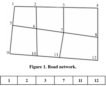
The GA design involves several key components: genetic representation, population initialization, fitness function, selection scheme, crossover, and mutation. A sample road network is shown as in Figure 1. The objec-tion is to find the optimum route from source node 1 to destination node 12. The GA method can be described as follows.

1) Genetic representation

A routing path from source node to the destination node is encoded by a string of positive integers that rep-resent the IDs of nodes through which the path passes. Each position of the string represents an order of the node in the road network. A feasible route is from the source node to the destination node without circle. Fig-ure 2 is a sample from source node to the destination node.

2) Population initialization

The initial population P is composed of a certain

number of chromosomes. The source node is taken as the starting point of a chromosome , which is constant. A feasible route is generated though selecting one of the neighbors provided that it has not been picked before. It keeps doing this operation until it reaches to destination node. The population scale is determined according to practical requirement.

p

3) Fitness function

[image:3.595.318.529.551.722.2]

For a given solution, evaluate its quality, which is determined by the fitness function. In this paper, the fitness function is the probability of arriving at destination in time . The probability distribution of a given solution t

Figure 1. Road network.

1 2 3 7 11 12

(4)

is calculated according to (13). 4) Crossover and mutation

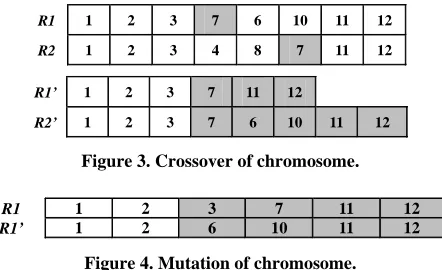
The single-point crossover is supposed to exchange partial chromosomes. With the crossover probability, each time we select two chromosomes i and j for crossover. They should possess at least one common node. The crossover process is shown as in Figure 3. After selection and crossover the population will undergo the mutation operation.

r r

With the mutation probability, each time we select one chromosome i on which one gene is randomly selected as the mutation point. The mutation will replace the sub path by a new random sub path. Mutation process is shown as in Figure 4.

r

5) Selection

After crossover and mutation, initial and new generated chromosomes are used for selection. The chromosome with high fitness value has great chance to be cop- ied to the next generation.

Repeat the process until terminating condition is reached.

5. Examples

One year GPS floating car data of 3500 taxis are provided by Jinan Urban Public Passenger Transport Man- agement Services Center. In the aggregation of GPS floating car data, the upload interval is set 20 seconds. The uploaded record items include vehicle’s running speed, direction, longitude, latitude et al. parameters. The

lon-gitude, latitude, direction parameters are used to locate the vehicle position with map matching method. The probability of the traffic state is analyzed with the proposed method. The selected road network is shown as in Figure 1. The time interval between two analyses is 5 minutes. The traffic flow data from 8:00 to 8:05 are selected.

5.1. Data Processing

Firstly, we will make the map matching according to the GPS floating car data. The data that are invalid to analyze traffic flow are deleted. They are recovered with forecasting method. In this example, exponent smoothing

R1 1 2 3 7 6 10 11 12

R2 1 2 3 4 8 7 11 12

R1’ 1 2 3 7 11 12

[image:4.595.62.283.600.735.2]

R2’ 1 2 3 7 6 10 11 12

Figure 3. Crossover of chromosome.

R1 1 2 3 7 11 12

R1’ 1 2 6 10 11 12

Figure 4. Mutation of chromosome.

method is used to forecast missing or deleted running GPS floating car data.

5.2. Travel Time Calculation

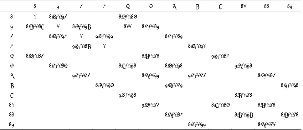
Travel time is estimated with (3) according to each floating car. The probability distributions of travel time of the road section corresponding to each time section are estimated with Bayesian method. The obtained distribution parameters of each time section are listed in Table 1.

5.3. Optimum Route Calculation

Use the improved GA method of section 4 to find the optimum path. The parameters of GA are set as follows. The initial population number is set 5 and generated chromosomes are shown in Figure 5. The crossover rate and mutation rate are set 0.4 and 0.1 respectively. The iteration threshold value is set 20. When , the optimum route is

10

t 11 1 1 2 3 7 2 opt

R     

7

t 2 3 4 8 12

 whose probability is 0.97. When , the optimum route is

opt 1

R       whose probability is 0.31.

5.4. Results Analysis

From the example’s analysis results we can find that the optimum route based on stochastic travel time can be obtained with the proposed method. When the desired travel time is different, the optimum route is different also.

6. Conclusion

Optimum path based on random travel time is an important problem. The optimum path finding method proposed in this paper is based on stochastic travel time, which can describe the real traffic situation properly. The probability of arriving at destination point in desired time is taken as the objection function. Classic optimum path finding methods, Dijkstra’s algorithm and A*_{, are not}

suitable to be used to solve the optimum path problems. In this paper, an improved genetic algorithm is adopted to solve the optimum problem. From the practical example analysis results we can find that the proposed method is efficient in dealing with optimal path problem. GPS floating car has been widely adopted. It is possible to

[image:4.595.311.534.637.725.2]

R1 1 2 6 10 11 12 R1 1 5 6 7 8 12 R1 1 2 6 5 9 10 11 12 R1 1 2 3 7 6 10 11 12 R1 1 2 3 4 8 7 11 12

(5)

[image:5.595.57.541.108.315.2]

Table 1. Probability distribution parameters of road network



 2



, .

1 2 3 4 5 6 7 8 9 10 11 12

1 0 1.5, 0.23 ∞ ∞ 1.6, 0.16 ∞ ∞ ∞ ∞ ∞ ∞ ∞

2 1.8, 0.19 0 1.7, 0.28 ∞ 100 1.4, 0.12 ∞ ∞ ∞ ∞ ∞ ∞

3 ∞ 1.6, 0.24 0 2.1, 0.22 ∞ ∞ 1.4, 0.12 ∞ ∞ ∞ ∞ ∞

4 ∞ ∞ 2.2, 0.18 0 ∞ ∞ ∞ 1.6, 0.20 ∞ ∞ ∞ ∞

5 1.5, 0.13 ∞ ∞ ∞ ∞ 1.8, 0.31 ∞ 2.2, 0.14 ∞ ∞ ∞

6 ∞ 1.4, 0.15 ∞ ∞ 1.9, 0.21 ∞ 1.6, 0.21 ∞ ∞ 2.7, 0.21 ∞ ∞

7 ∞ ∞ 2.4, 0.33 ∞ ∞ 1.7, 0.22 2.4, 0.33 ∞ ∞ 1.6, 0.13 ∞

8 ∞ ∞ ∞ 1.7, 0.26 ∞ ∞ 2.5, 0.32 ∞ ∞ ∞ ∞ 1.2, 0.21

9 ∞ ∞ ∞ ∞ 2.1, 0.21 ∞ ∞ ∞ ∞ 1.8, 0.31 ∞ ∞

10 ∞ ∞ ∞ ∞ ∞ 2.5, 0.33 ∞ ∞ 1.9, 0.16 ∞ 1.8, 0.31 ∞

11 ∞ ∞ ∞ ∞ ∞ ∞ 1.7, 0.14 ∞ ∞ 1.8, 0.28 ∞ 1.8, 0.31

12 ∞ ∞ ∞ ∞ ∞ ∞ ∞ 1.3, 0.22 ∞ ∞ 1.7, 0.30 ∞

Note: ∞ denotes that the two node are not connected directly.

apply the proposed method to practical system. With the development of floating car, the data scale will become larger and larger. How to extend the proposed optimal path finding method to large scale data is our future research work.

7. Acknowledgements

This work is partially supported by national youth science foundation (No. 61004115), national science foundation (No. 61272433), and Provincial Fund for Nature project (No. ZR2010FQ018)

REFERENCES

[1] Y. Nie and Y. Y. Fan, “Arriving-On-Time Problem: Dis- crete Algorithm That Ensures Convergence,” Transporta- tion Research Record, 1964, pp. 193-200.

[2] E. W. Dijkstra, “A Note on Two Problems on Connexion with Graphs,” Numerische Mathematik, Vol. 1, No. 1, 1959, pp. 269-271.

http://dx.doi.org/10.1007/BF01386390

[3] M. Sniedovich, “Dijkstra’s Algorithm Revisited: The Dynamic Programming Connexion,” Journal of Control and Cybernetics, Vol. 35, No. 3, 2006, pp. 599-620. [4] R. W. Floyd, “Algorithm 97: Shortest Path,” Communi-

cations of the ACM, Vol. 5, No. 6, 1962, p. 345.

http://dx.doi.org/10.1145/367766.368168

[5] R. Bellman, “On a Routing Problem,” Quarterly of Ap-plied Mathematics, Vol. 16, No. 1, 1958, pp. 87-90. [6] D. Delling, P. Sanders, D. Schultes and D. Wagner, “En-

gineering Route Planning Algorithms,” Algorithmics of Large and Complex Networks, Vol. 5515, 2009, pp. 117- 139.http://dx.doi.org/10.1007/978-3-642-02094-0_7 [7] P. E. Hart, N. J. Nilsson and B. Raphael, “A Formal Basis

for the Heuristic Determination of Minimum Cost Paths,” IEEE Transactions on Systems Science and Cybernetic, Vol. 4, No. 2, 1968, pp. 100-107.

http://dx.doi.org/10.1109/TSSC.1968.300136

[8] I. Chabini, “Discrete Dynamic Shortest Path Problems in Transportation Applications: Complexity and Algorithms with Optimal Run Time,” Transportation Research Re- cord, Vol. 1645, No. 1, 1998, pp. 170-175.

http://dx.doi.org/10.3141/1645-21

[9] Y. Fan, R. E. Kalaba and J. E. Moore, “Shortest Paths in Stochastic Networks with Correlated Link Costs,” Com- puters and Mathematics with Applications, Vol. 49, No. 9-10, 2005, pp. 1549-1564.

http://dx.doi.org/10.1016/j.camwa.2004.07.028

[10] E. D. Miller-Hooks and H. S. Mahmassani, “Least Ex- pected Time Paths in Stochastic, Time-Varying Trans- portation Networks,” Transportation Science, Vol. 34, No. 2, 2002, pp. 198-215.

http://dx.doi.org/10.1287/trsc.34.2.198.12304

[11] Z. S. Yang, “Basis Traffic Information Fusion Technol- ogy and Its Application,” China Railway Publish House, Beijing, 2005.

[12] C. Liu, X. L. Meng and Y. M. Fan, “Determination of Rou- ting Velocity with GPS Floating Car Data and WebGIS- Based Instantaneous Traffic Information Dissemination,” The Journal of Navigation, Vol. 61, No. 2, 2008, pp. 337- 353.http://dx.doi.org/10.1017/S0373463307004547 [13] X. Zhang, “Shortest Path’s Probability Distribution of

Stochastic Road Network,” Master Thesis, 2010.

[14] P. B. Mirchandani, “Shortest Distance and Reliability of Probabilistic Networks,” Computer and Operations Re-search, Vol. 3, No. 4, 1976, pp. 347-355.

http://dx.doi.org/10.1016/0305-0548(76)90017-4

(6)

[16] G. R. Jagadeesh, T. Srikanthan and K. H. Quek, “Heuris- tic Techniques for Accelerating Hierarchical Routing on Road Networks,” IEEE Transactions on Intelligent Trans- portation Systems, Vol. 3, No. 4, 2002, pp. 301-309.

http://dx.doi.org/10.1109/TITS.2002.806806

[17] C. W. Ahn and R. S. Ramakrishna, “A Nondominated Sorting Genetic Algorithm for Shortest Path Routing Pro- blem,” IEEE Transactions on Evolutionary Computa- tion, Vol. 6, No. 6, 2002, pp. 566-579.