http://www.scirp.org/journal/jhepgc ISSN Online: 2380-4335 ISSN Print: 2380-4327
DOI: 10.4236/jhepgc.2018.42019 Apr. 27, 2018 262 Journal of High Energy Physics, Gravitation and Cosmology
Measurement Quantization Unites Classical and
Quantum Physics
Jody A. Geiger
Informativity Institute, Chicago,Illinois, USA
Abstract
Unifying quantum and classical physics has proved difficult as their postulates are conflicting. Using the notion of counts of the fundamental measures—length, mass, and time—a unifying description is resolved. A theoretical framework is presented in a set of postulates by which a conversion between expressions from quantum and classical physics can be made. Conversions of well-known expressions from different areas of physics (quantum physics, gravitation, op-tics and cosmology) exemplify the approach and mathematical procedures. The postulated integer counts of fundamental measures change our under-standing of length, suggesting that our current underunder-standing of reality is dis-torted.
Keywords
Gravity, Gravitational Constant, Planck’s Constant, Planck Units, Hubble’s Constant, Momentum, Quantum Uncertainty, Dark Energy, Dark Matter, Cosmic Microwave Background
1. Introduction
On the nature of electromagnetic radiation (ER) and its unique properties in re-lation to blackbody spectral emissions, Planck’s work introduced the notion of quantized energy packets that led to a better understanding of light. He post-ulated that ER adhered to a strict quantal rule in the absorption and emission rules with photon energies given by E = nhv where n is the number of packets, h is Planck’s constant, and v is frequency [1]. The constant h was later understood as the smallest action that could exist in nature and with it, Planck developed expressions for the fundamental units of length, mass, and time:
1 2
3 m
p
G l
c =
[2] [3],
(1)
How to cite this paper: Geiger, J.A. (2018) Measurement Quantization Unites Classic-al and Quantum Physics. Journal of High Energy Physics, Gravitation and Cosmolo-gy, 4, 262-311.
https://doi.org/10.4236/jhepgc.2018.42019
Received: January 26, 2018 Accepted: April 24, 2018 Published: April 27, 2018
Copyright © 2018 by author and Scientific Research Publishing Inc. This work is licensed under the Creative Commons Attribution International License (CC BY 4.0).
http://creativecommons.org/licenses/by/4.0/
DOI: 10.4236/jhepgc.2018.42019 263 Journal of High Energy Physics, Gravitation and Cosmology 1 2
5 s
p
G t
c =
[2] [3], (2)
1 2
kg
p c m
G
= [2] [3]. (3) Planck’s formulation is built on a nondimensionalized framework of funda-mental units of measure and succeeds in revealing important fundafunda-mental rela-tionships, but does not establish a grounded understanding of their significance. The values, lp, mp and tp are derived from measures of ħ, G and c. Because the values are interpreted to represent a smallest measure, we may infer that they can never be directly measured. To do so, it would imply an ability to measure a value by means of physical elements that were equal or larger than the target. There has been no significant progress addressing this issue since Planck’s initial publication.
In this paper, we will present experimental data that demonstrate the physical significance of these measures. The approach departs from modern theory with a view that the underlying reference frame adheres to rules which are more dis-crete than quantum. This opposing perspective, a model based on a background independent framework [4] of discrete indivisible units of length, mass and time, is what separates this approach. Referred to as Informativity, this model is an approach based on the idea that phenomena are described as discrete units, that is, integer values of a fixed amount of measure. Observations of light are consi-dered in geometric terms that may be used to describe gravity, dark energy, visi-ble and observavisi-ble mass, inflation, the big bang and the cosmic microwave background (CMB) as a whole-unit interpretation of physical phenomena.
The model parallels modern theory, in design, as it is similar in principle to that taken by Albert Einstein. Einstein’s model for special relativity (SR) arises from an understanding that the speed of light lp/tp is a physically significant bound. This model recognizes that mp/tp is a physically significant bound.
With the model, we present a fundamental expression that relates length, mass and time. For each measure, the expression is at best a composite of the other two. Self-referencing measures (i.e. measures defined in terms of other measures) provide a framework for developing expressions of observed pheno-mena. However, when working with dark energy, a difficulty arises in under-standing phenomena that are properties of the universe. This research recogniz-es where phenomena “within” the system are understood with rrecogniz-espect to the self-referencing measurement framework then phenomena that are properties “of” the system are understood with respect to a self-defining measurement framework.
DOI: 10.4236/jhepgc.2018.42019 264 Journal of High Energy Physics, Gravitation and Cosmology evidentiary support for the physical significance of fundamental units, a demon-stration of the relationship between Planck’s units and the fundamental units of measure, a calculation of Hubble’s constant, the age, size, mass and density of the universe, how much matter is visible, observable and what can never be ob-served. Expressions describing expansion, dark energy and dark matter are also presented and explained.
In the process of resolving an understanding of mass, we also present new ex-pressions describing the birth of the universe, what starts and stops inflation (which we will distinguish from the modern understanding of inflation with the term, quantum inflation), what causes the big bang and the underlying mechan-ics that cause expansion. To validate the approach, among other outcomes, the model is used to calculate the age, energy, density and temperature of the CMB and present an understanding of the processes that constrain those values. A study of CMB measurements confirms the results to four significant digits, our best measurement data available.
In addition to cosmological phenomena, Informativity also allows for the de-velopment of expressions in quantum physics. For one, using a Bell state model presented by Shwartz and Harris [5], expressions are presented that describe the presence of a distorting effect at work in the measure of G and ħ. Understanding this effect leads to the resolution of contradictions in the evaluation of certain expressions and provides a foundation with which to develop expressions that describe phenomena both very large and very small.
2. Methods
The approach is based on the idea that three fundamental measures may be rela-tively defined: length, mass, and time. The measures are identified by symbols lf, mf, and tf, but at this stage are not assigned values. The subscript f is used to dis-tinguish the fundamental measures of Informativity from Planck’s units, Equa-tions (1)-(3).
Although the values of lf and tf are unspecified, their ratio may be understood and constrained by the elapsed time on an atomic clock relative to a distance traveled by a pulsed laser beam in vacuo, where c = lf/tf with respect to any iner-tial frame. It is recognized that this ratio is fixed given the experimental support for the invariance of the value of c. Where nLflf= nTftfc, a count of lf, i.e., nLf, will equal a count of tf, i.e., nTf. Note that lf or tf may take any value and as such an arbitrary value may be chosen such that it is the largest value for which no smaller value can be observed. Other physical quantities, in turn, are obtained as counts of the fundamental measures.
DOI: 10.4236/jhepgc.2018.42019 265 Journal of High Energy Physics, Gravitation and Cosmology Note that time has been subtly tied to distance and for that reason our defini-tion is not only inclusive of the three spatial dimensions but extends to the tem-poral dimension. Without time, there exists no means to define space.
We summarize these two statements, which with two others formalize our model:
O1: Quantities exist which are whole-unit counts of the fundamental measures lf and tf.
O2: Mass may be a whole or fractional count of mf.
O3: Any remainder of a whole-unit calculation of lf or tf describes an action. O4: Distances for which the Pythagorean Theorem applies, the shortest side a is fixed with a count of one lf, against which counts of lf along sides b and c are made.
An underlying premise of the model is that in O1 and O2 all measures are de-fined relatively. With a unit system applied, there exists an agreed upon frame-work by which phenomena may be described by counting fundamental meas-ures. O3 recognizes the possibility that some expressions may solve for fractional counts of fundamental measures. Fractional counts violate the premise by which lf and tf are established. Therefore, any expression that describes a change in dis-tance equal to the remainder of a measure must also describe an action.
O4 presents a tool, the Pythagorean Theorem, for estimating length. Where the measure is relatively defined, the theorem incorporates a reference which must be equal to a unit count of one; that is a = 1 unit is the reference. The other short side b is any given unit count of distance measures whereas the long side c (hypotenuse) is the distance measure of unknown unit count. Each side is a count of the reference measure defined by a. This establishes a foundation for a background independent framework that acknowledges the need for a reference within the definition. The expression 12 + b2 = c2 describes an unknown distance c relative to b in terms of a count of a. As desired, solutions to c result in values that are fractional leaving us to test the hypothesis that gravity may be described as the lost excess over and above the whole-unit count of distance measures.
While we recognize that the measurement of quantities is limited, this does not mean they are not significant. Validating their significance against existing data is one goal of the model. Furthermore, although we use the Pythagorean Theorem to understand distance, there is no specific argument to suggest that another geometric expression would not serve the same purpose. The theorem provides insight only so long as it allows the presentation of expressions that cannot be reduced by another means. Finally, the term fundamental was chosen as a general term with the connotation that a measure has the characteristic of being countable and that measurement may be characterized as a count of fun-damental measures. The term also serves to distinguish the units of measure adopted by Informativity from those given in Planck’s base system.
DOI: 10.4236/jhepgc.2018.42019 266 Journal of High Energy Physics, Gravitation and Cosmology the fundamental measures that are resolved entirely within Informativity.
3. Results
3.1. Length Measurement and Gravitational Acceleration
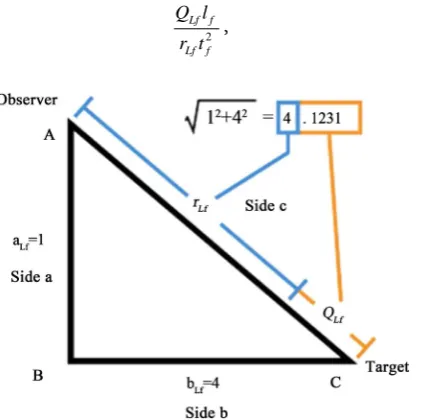
For long side c and short sides a = 1 and b of any chosen integer count of a right-angle triangle (Figure 1), we may resolve a count for the length measure representing the uncertain distance,
(
)
1 22
1 Lf
c= +b (4) Any non-whole-unit count relates to a change in distance and may be de-scribed by rounding up (repulsion) or down (attraction). The remainder lost to rounding will be denoted by QLf. For all solutions, QLf is less than half and thus attractive. An example of repulsion will be explored in the Section 3.13. The model provides a count of distance measures that is closer by
(
2)
1 21
Lf Lf Lf
Q = +b −b ,
(5) at every instant in time. For example, if bLf =4, then
(
17 4)
4 0.1231 4Lf Lf
Q r = − = . Because side c always rounds down, we find that rLf always equals bLf. In the following, we shall always refer to the “ob-served measure count” as rLf. Moreover, note that the reference measure against which all counts are measured is defined by aLf = 1. With this we have composed an expression for gravity such that the loss of the remainder rela-tive to the whole-unit count is QLf/rLf.
Together QLf and rLf are conjectured to represent an important dimension-less ratio that describes gravity. We proceed with that hypothesis by present-ing the ratio in meters per second squared (m/s2), where we multiply by l
f for meters and divide by 2
f
t together describing the distance loss at the maxi-mum sampling rate of one sampling every tf seconds per second,
2
Lf f
Lf f Q l
[image:5.595.272.496.496.706.2]r t , (6)
DOI: 10.4236/jhepgc.2018.42019 267 Journal of High Energy Physics, Gravitation and Cosmology We now note that this quantity is scaled and hence requires a scaling con-stant; we multiply by the speed of light c and divide by a scaling constant S. Setting r = rLflf and c = lf/tf, Equation (6) reduces to
2 2 3
2
Lf f Lf Lf f Lf
Lf f Lf f f
Lf f
Q l c Q c Q l c Q c
S r t S r l t S rS
r t = = = , (7) As the ratio c/S may be understood as 1/kg or a maximum count of mf per kilogram, it may also be thought of as the corresponding mass frequency as-sociated with gravity. Where S = 3.26239, this expression is now equivalent to G/r2 to five significant digits for all distances greater than 103l
f. Where quan-tum differences are not a consideration, we may set Equation (7) equal to G/r2 and therefore
3 2
Lf
Q c G
rS =r , (8) 3
Lf
Q rc =GS.
(9) We may interpret S as momentum; hence the units for these expressions will match accordingly. Nevertheless, recognizing that S is a dimensionless scalar is an important and critical detour that shall be central to the discus-sion below. Two applicable interpretations will be shown. We first investigate S as a momentum, and then perform a similar analysis as an angular measure.
Consider Equation (9); after rearranging and reducing the term on the right with r = rLflf, we use limb→∞ f Q r
(
Lf Lf)
=1 2 as noted in Appendix A. Inpassing, the term QLfrLf, referred to as the Informativity differential, plays a key role in describing how fractional values less than the theoretical limit de-scribe a distorting effect in measurement. Consideration of the Informativity differential at a limit is a matter of convenience, but to maintain a precise ex-pression, values for QLf and rLf should always be entered specific to the phe-nomenon being observed. The values determined can cover the entire physi-cal regime from one lf to infinity. From Equation (9), we have
3 2
Lf Lf Lf f f
c S S S
G =Q r=Q r l = l .
(10)
Multiply both sides by tf and reduce to obtain a mass,
3 2
kg
f f f
f
c S S
m t t
G l c
2
= = = . (11) Hence the momentum of a fundamental measure of mass (light) moving at c may be expressed as
1
2 kg m s 2
f S
m c c S
c
ρ= = = ⋅ ⋅ −
. (12) We understand S as being half the momentum of a fundamental measure of mass. This may also be written as
1
2 f f f kg m s
f m l
S m c
t
−
DOI: 10.4236/jhepgc.2018.42019 268 Journal of High Energy Physics, Gravitation and Cosmology Any count of lf must equal the count of tf, hence requiring that S must cor-respond to mf being fractional. There exists no prerequisite that Informativity expressions be composed of whole-unit counts of mf; see O2 of Section 2. With this resolved, we now consider S as an angular measure. With the Py-thagorean Theorem supporting an understanding of S as momentum, then a circle supports an understanding of S as an angle.
Consider Equation (1) organized such that 3 2
f
c G= l . Take Equation (10), replace c G3 with 2
f
l
and replace =h 2π. Hence
3
2
2 2 2 4π
f f
f f
f
h
l c l
S
G l l l
= = = =
, (14)
where S = ħ/2lf, then the arc length of a circle of radius lf and angle S is
2 2
f f
L l
l rθ= =
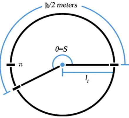
= . (15) In Figure 2, we find that an arc-length with θ = 2S radians is precisely the value of ħ as meters. Each of the terms has a suitable geometric description: • lf radius of a fundamental circle in meters,
• 2S angle in radians that subtends a segment with an arc length of ħ meters, • ħ arc-length of a segment corresponding to the momentum of a
funda-mental Measure of mass.
Applicability to an existing geometric expression is just the first of several tests. Next, we consider support for the equivalence of these two interpreta-tions. We begin by resolving S in terms of our initial description of gravity from Equation (10),
3
1
kg m s 2
f
l c S
G
−
[image:7.595.264.484.508.709.2]= ⋅ ⋅ . (16) Next consider S = ħ/2lf as resolved in Equation (14). With lfc3/2G a mo-mentum and ħ/2lf an angular measure, we set them equal giving
DOI: 10.4236/jhepgc.2018.42019 269 Journal of High Energy Physics, Gravitation and Cosmology 3
2 2
f
f
l c
G = l
. (17)
Isolating lf to the left-hand side and
1 2
3 m
f G l
c
= [2] [3].
(18) The expression clarifies our conjecture of the equivalence between the two interpretations: momentum and angular measure. The expression also de-monstrates that the comparison is in fact a modified form of Planck’s univer-sally recognized formulation for length.
Finally, to verify this interpretation, we now seek a quantity where S is: • An invariant characteristic of light at a threshold,
• Described as lfc3/G with respect to momentum, • Described as ħ/2lf with respect to angular measure.
A quantity was measured by Shwartz and Harris in 2011 regarding the quantum entanglement of light at the degenerate state [5]. Using polarization entangled photons in pure Bell states at X-ray wavelengths, they were able to take advantage of the intersections of the component curve (as a function of the square of the current density) to resolve pump angles θp where the mag-nitudes of the components of each Bell state are equal. With this, solutions to the phase matching and current density equations were resolved to determine the sign of the components at the intersection. Then solving the phase matching equations for the signal θs and idler θi with respect to the atomic planes, substituting the related electric fields, the current density is a function of just the pump angle. With these conditions in place, the momentum of a fundamental measure of mass is then equal in value to the angle of the signal and idler lfc3/2G with respect to the atomic planes where the pump is at its maximum angle.
There are five pump angles representing two of the Bell states that can generate entangled photons and lfc3/2G is uniquely distinguished where θp is at its maximum. Shwartz and Harris recognize these Bell states, where H
is the polarization of the electric field of the X-ray in the scattering plane and
V is the polarization orthogonal to the scattering plane which contains the
incident k vector and the lattice k vector G. Subscripts p, s, and i, respectively, denote the pump, signal and idler.
The expressions in Table 1 arise from Equation (16) each describing an equidistant angle either side of 0, π or 2π and are precisely identical in value to the Shwartz and Harris measurements. Using the most recent CODATA [2] as a guide for the value of lf, we find that
(
)
335 3
11
1.616199 10 299792458
3.26239 radians
2 2 6.67408 10
f l c S
G
−
−
× ×
×
= =
×
= .
(19)
But, where we have made use of Planck’s relation in Equation (14),
2 f 3.26250
DOI: 10.4236/jhepgc.2018.42019 270 Journal of High Energy Physics, Gravitation and Cosmology
Table 1. Angle setting in radians of the k vectors of the pump, signal and idler for
maximally entangled states at the degenerate frequency with corresponding Shwartz and Harris values (Reference [5]).
Bell’s State k vector angle
θp θs θi
(
H Vs, i +V Hs, i)
2 (lfc3/2G)− π (0.1208) π − (lfc3/2G) (−0.1208) π − (lfc3/2G) (−0.1208)2π − (lfc3/2G) (3.02079) (lfc3/2G) (3.26239) (lfc3/2G) (3.26239)
Informativity precisely matches the values presented in the Shwartz and Har-ris model, but our understanding of ħ when applying Planck’s expression is incomplete. The issue that affects Planck’s reduced constant will be resolved in Section 4.
The correlation between S and the angular measures of the Shwartz and Harris Bell state is not unexpected. Where the signal and idler are resolved specifically to obtain the polarization angles necessary for entanglement, seeking the pump angle follows naturally, thereby resolving each of the con-ditions where entanglement may occur. Informativity is not a coincidental alignment of one of these values, but a means of resolving the maximum an-gular measure corresponding to light in terms of the fundamental measure mf. With that, resolving the angular measures for each of the limits described by the Bell state follows in a straight-forward manner.
Where the expression 2S describes the momentum of a fundamental meas-ure of mass, the term S describes an angle. Both interpretations are valid. The juxtaposition of units describes a relationship that is conflicting, similar to Einstein’s relation E = mc2, which expresses energy in joules as a form of mass in kilograms, and vice versa. This presentation demonstrates that momentum and angular measure are one and the same.
With this understanding we consider replacing the scalar term S with θsi. The term alludes to recognizing the angular measure of the signal and idler under some conditions and momentum under others. Although both inter-pretations are applicable, θsi is retained emphasizing that we are not working with a theoretical value, but an invariant macroscopic measure. Additional research regarding the measure of θsi has been reported [6], where the error in angular measurement is estimated to be less than 2 micro-radians.
DOI: 10.4236/jhepgc.2018.42019 271 Journal of High Energy Physics, Gravitation and Cosmology One might also view this approach as an innovative alternative to Newto-nian vector calculus thus side-stepping what might be an otherwise tradition-al understanding of gravitation. However, this argument would tradition-also work against an underlying premise of this paper, that higher-order operators (other than the four basic arithmetic operators) disguise the fundamental constructs. Where a treatment using vector calculus would resolve the tradi-tional presentation, the quantum relationship to θsi would be lost or at least well-disguised.
3.2. Fundamental Measures
With the θsi correlation, we may now resolve the fundamental measures lf, mf, and tf, not as a theoretical construct, but with physical expressions constrained by the characteristics of light and gravity, consisting entirely of macroscopic measures. We start with Equation (10) by solving for lf,
(
)
11
35
3 3
2 2 6.67408 10 3.26239
1.61620 10 m
299792458 si
f
G l
c
θ
−−
× × ×
= = = × , (20)
where time follows from the definition tf = lf/c. Replacing lf with Equation (20) gives
(
)
11
44
4 4
2 2 6.67408 10 3.26239
5.39106 10 s
299792458
f si
f
l G
t
c c
θ
−−
× × ×
= = = = × . (21)
Finally, reordering time to resolve mass
3
8
2 2 3.26239
2.17643 10 kg 299792458
si
f f
c
m t
G c
θ × −
= = = = × ,
(22)
where interpreting S = θsi as a momentum yields the appropriate units. Most importantly, whereas the value for θsi is obtained from a macroscopic measure-ment, Planck’s approach is achieved as a theoretical construct. Establishing that these values are the same provides a new foundation with which to build a mod-el based entirmod-ely on physical measurements. Also note, whereas lf and tf are pro-posed to be the smallest significant measures, mf is not; mf does play a central role in many expressions because it is a product of lf and tf, i.e.mf= 2θsitf/lf, and for that reason the term is retained.
The Informativity formulation parallels Planck’s although the expressions are presented in quantized terms and are entirely formulated under the background independent framework of Informativity. An additional characteristic of the fundamental measures is that they are not a product of Planck’s formulations, Planck’s constant or any quantum term. Rather, values are derived using only the geometric expression 3
Lf si
Q =G
θ
rc . The expression depends on c, r, G and θsi and all are resolved macroscopically. Where r=r lLf f and(
)
limr=∞ f Q rLf Lf =1 2 from Appendix A, the relation is rearranged to give
(
3)
2
si lf c G
DOI: 10.4236/jhepgc.2018.42019 272 Journal of High Energy Physics, Gravitation and Cosmology Planck’s approach provides a valid way to constrain the fundamental meas-ures, but the solution provides no mechanism to confirm the approach through measurement indirectly confirming the significance of the measures. The Infor-mativity approach recognizes the significance of θsi and uses that to resolve lf, mf, and tf. Whereas both approaches arrive with the same conclusion, the ability to resolve the fundamental measures as a product of macroscopic phenomena is an important and decisive difference.
It should finally be noted that the fundamental measures lf and tf can never be directly resolved with identical or greater precision. This would defy their defini-tion. The fundamental measures are the references against which everything is de-fined. It would be neither possible nor meaningful to measure a reference where the most appropriate reference is the reference itself. Fundamental measures can only be inferred as a characteristic of nature that indicates their significance.
3.3. Newton’s Constant
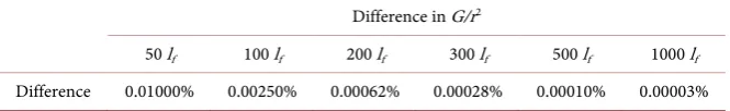
Using Equation (8) at the quantum scale to calculate G will show a difference with Newton’s presentation. Is G variable [7]? No. The difference is a reflection of the precision between the geometric model of Informativity in comparison to Newton’s presentation. Newton’s expression does not include the geometric distortion effect inherent in the Informativity differentialQLfrLf as numerically assessed in Table 2.
For clarity, we work through a calculation. A distance of 1 meter is intention-ally selected such that G r2 =G1=G. Using Equation (20) for l
f, the inverse gives us a count in 1 meter such that 34
6.18735 10
b= × ; that is,
2
1
Lf
Q = − =c b +b −b, (23)
(
34)
2 34 366.18735 1
1 6.18735 10 0 8.08100 10
Lf
Q = + × − × = × − ,
(
)
33 36
11 2
8.08100 10 299792458
6.67407 10 m kg s
1 3.26239 Lf
si
Q c
r
θ
−
−
× ×
= = × ⋅
× . (24)
[image:11.595.208.541.667.718.2]With only our understanding as prescribed by the Pythagorean Theorem and expressed in Equation (7), this is G/r2 at a distance of 1 meter, and therefore numerically equal to G. The formulation depends on an understanding of lf, which may be resolved from the expression presented in Equation (20). The value is also identical to the most recent CODATA estimate of Planck’s formula-tion of length. The CODATA [2] [8] estimates of Planck units have changed over recent years, but those estimates continue to give support to the expressions
Table 2. Informativity difference in G/r2.
Difference in G/r2
50 lf 100 lf 200 lf 300 lf 500 lf 1000 lf
DOI: 10.4236/jhepgc.2018.42019 273 Journal of High Energy Physics, Gravitation and Cosmology of Informativity.
While Informativity does provide a concise geometric expression for G, the term may also be understood as a physically significant product of two limits.
To understand, we will need more formal definitions for the fundamental lim-its. Begin by considering time as a convenient measure with which to better un-derstand length and mass. We may then ask what is the upper limiting relation of lf and mf with respect to time, tf?
8
2.99792458 10 m s
f f
l t = × ,
(25) 35
4.0371111 10 kg s
f f
m t = × . (26) The first expression embodies the number of meters traversed by light in a second. Similarly, the second expression embodies the number of kilograms that may be traversed in a second. By implication, each describes the maximum rate of change that may be observed in one measure relative to the other measure.
As such, we may interpret lf/tf as an upper bound to speed; such an interpreta-tion is quite valid. Nevertheless, the focus of the expression is that the value is an upper bound to this observation. In a system with a fixed rate of change 1/tf and an upper bound to the observation of units of lf per tf, once that bound is reached, the observer can no longer distinguish a greater number of events. To do so would violate our understanding of the fundamental measures of length and time implying that we would be able to observe measures smaller than the fundamental measures. Moreover, it is not that physical phenomena cannot overlap in space-time, but that an observer has a specific upper bound to the number of events that may be distinguished.
Before we begin, note that up to this point we have distinguished counts of Planck units (i.e. nLp) from the fundamental units of Informativity (i.e. nLf). Moving forward, all counts that reference fundamental units and will not carry the subscript f following the designated measure. The only exception to this rule will be components of the Informativity differential, QLfrLf.
To express a count of lf, mf and tf, we would divide the rate by the respective unit measure.
8 43
2.99792458 10 1.85492 10 units s
L f
n = × l = × ,
(27)
35 43
4.0371111 10 1.85492 10 units s
M f
n = × m = × , (28)
43
1 1.85492 10 units s
T f
n = t = × , (29) Thus, observe that
O5: A count of each of the fundamental measures with respect to any shared measure is the same.
L T M
DOI: 10.4236/jhepgc.2018.42019 274 Journal of High Energy Physics, Gravitation and Cosmology second. The comparison brings to our attention that change is constrained. For all measures, there exists a maximum frequency such that a target may have: • A maximum length frequency of lf/tf,
• A maximum mass frequency of mf/tf and, • A maximum count frequency of 1/tf.
Where G is expressed in terms of maximums such that
3 3 3 3
3 2
kg s 2
Lf Lf Lf f f f f f f f
si si si f f f f f
Q rc Q r l c c l c t l l l t
G m
m t t t m
θ
θ
θ
= = = = = ⋅ , (31)
we now recognize that Newton’s expression is a formal description of the maxi-mum rate of change in space (i.e. the three dimensions) with respect to (i.e. di-vided by) the maximum rate of change in mass. In that there are no other com-binations of the fundamental measures with respect to space, we find gravity a unique and singular phenomenon for which there are no other examples.
To further our understanding of gravitation, consider a cube with sides meas-ured in terms of lf equal to the distance that light travels per second. We find that this cube contains a count of c3 units of daughter cubes, each having sides equal to lf. The parent cube provides a grid-like understanding of an inertial frame describing the maximum frequency of lf relative to tf.
Next, consider mf/tf as a scalar quantity defining a count of mass units—the maximum mass frequency—that may exist along the edge of the parent cube. Thus, dividing the cubic length frequency (lf/tf)3 by the mass frequency mf/tf gives a fixed relation for mass relative to an observer in space; in other words, this is the most appropriate understanding of the gravitational field relative to an inertial frame.
We expand on this approach by also noting that, where G expresses a property of gravity, then the speed of gravity, sgravity, may be resolved by a process of fac-toring out known components. First, multiply G by the mass frequency thereby removing the mass component. Next, reduce space-time by dividing the cubic length frequency in two of the three dimensions, c2, such that the linear speed of gravity is
gravity 2
1
m s
f
f m
s G
t c
c
=
=
.
(32)
DOI: 10.4236/jhepgc.2018.42019 275 Journal of High Energy Physics, Gravitation and Cosmology
3.4. Planck’s Constant
To build on our understanding of G presented in Section 3.3, we investigate how the use of macroscopic and quantum terms affects the calculation of physical measures. We begin by formulating a known Informativity expression that may serve as a reference. Dividing Equation (9) by G, substituting r = rLflf, and fac-toring c3/G, we obtain
3 3 3
3.26239 radians 2
Lf f
si Lf Lf f
Q rc c c l
Q r l
G G G
θ
= = = = . (33)
The measure for θsi matches the angular measurements made by Shwartz and Harris. We derived lf because of the correlation of S and θsi. Comparing Planck’s formulation in Equation (1) where 3 2
f
c G= l and substituting it into Equa-tion (33) yields
3
2 3.26250 radians
2
si Lf Lf f Lf Lf f
f f
c
Q r l Q r l
G l l
θ = = = =
, (34)
where G and r2 are macroscopic factors whereas ħ has a quantum origin; all val-ues of fundamental units, such as lf, are neither macroscopic nor quantum, but treated as constants. For convenience, the macroscopic limit of the Informativity differential is taken, and not its quantum limit. This is acceptable when working with macroscopic terms, but when working with quantum terms, including the Planck constant, that limit produces inaccurate results. The Informativity diffe-rential needs to be retained and expressions properly calculated regarding the actual distance of the measured interaction. With respect to the conditions that lead to the measure of ħ, distance as a count of lfmay be resolved by solving for rLf using its expression in Equation (C7) as derived in Appendix C,
(
1)
84.855362 Lf si f
si f
r l
l θ
θ =
− =
. (35)
Note that rLf must be a whole-unit count, 85lf. Resolving a quantum distance provides an understanding as to why Planck’s constant as it is currently defined is appropriate in expressions such as the fine-structure constant [9]. Hence, use of Planck’s reduced constant at an Informativity differential distance of 85lf produces the correct result. However, the expression is not appropriate in ex-pressions consisting entirely of macroscopic measures. With G, both factors vary depending on the Informativity differential.
We understand this effect better by solving for ħ using Equation (34) and then comparing that to the currently recognized value of 34
1.05457 10−
= ×
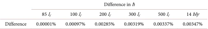
[2]. For this purpose, we see in Table 3 that the variation in ħ changes quickest within the first few lf.
DOI: 10.4236/jhepgc.2018.42019 276 Journal of High Energy Physics, Gravitation and Cosmology then
2
34
2 1.05454 10 J s
f si f si
si f Lf Lf f Lf Lf
l l
l
Q r l Q r
θ
θ
θ
−= = = = × ⋅
. (36)
With this value, the distance-adjusted Informativity and Planck formulations are now mathematically equivalent and the variation in G and ħ cancel out:
1 2
3 3
2
m si
G G
c c
θ
=
, (37)
1 2
4 5
2
s
si
G G
c c
θ
=
, (38)
1 2
2
kg
si c
c G
θ
= . (39) Each expression may be reduced to
2 3
4Gθsi=c (40)
where uncertainty exists in the derivation of lf, mf, and tf, we may express the fundamental measures in terms of θsi instead of ħ. This expression confirms that any geometric distortion in ħ is proportionally compensated with the same in G. We are also more aware of the important role played by the Informativity diffe-rential and have confirmed that these two very different approaches arrive at precisely the same result. Note further that this is a well-grounded physical ex-pression that may be used to resolve each of the fundamental measures, thus providing significance to each. Finally, with a distance adjusted value for ħ, we can return to the Shwartz and Harris results as presented in Table 1 and cast them in terms of the ratio of arc length and diameter of a circle.
With 34
1.05454 10− J s
= × ⋅
from Equation (36) and 35
1.61620 10 m
f
l = × −
[image:15.595.224.536.163.299.2]from Equation (20) (where their ratio corresponds to units in radians as resolved in Equation (15)), these expressions precisely match the Shwartz and Harris val-ues [5]. Whether presented in macroscopic or quantum terms, we find the an-gular measures presented in Table 4 may be resolved.
Table 3. Informativity difference in Planck’s reduced constant ħ.
Difference in ħ
85 lf 100 lf 200 lf 300 lf 500 lf 14 bly
Difference 0.00001% 0.00097% 0.00285% 0.00319% 0.00337% 0.00347%
Table 4. Angles in radians for the k vectors of the pump, signal, and idler for the
maximally engangled states at the degenerate frequency with corresponding Shwartz and Harris values (Reference [5]).
Bell’s State k vector angle
θp θs θi
(
H Vs, i +V Hs, i)
2 (ħ/2lf) − π (0.1208) π − (ħ/2lf) (−0.1208) π − (ħ/2lf) (−0.1208) [image:15.595.207.540.559.606.2]DOI: 10.4236/jhepgc.2018.42019 277 Journal of High Energy Physics, Gravitation and Cosmology
3.5. Fundamental Measures Correlated
In Equations (20)-(22), solutions to the fundamental measures are resolved and while they are appropriate for use in macroscopic terms, it is not representative of a distance-sensitive formulation. Here, we resolve distance-sensitive expres-sions and demonstrate their use in several well-known expresexpres-sions. We begin with Equation (11) and expand the right-hand term restoring the Informativity differential to mass that was factored out in Equation (10) with the limiting process (Appendix A),
2 si si
f
Lf Lf m
c Q r c
θ θ
= = . (41)
We may now translate mass to a length and time by applying the fundamental transforms (Appendix B) ∆
(
lf →mf)
where2
f f
l c G=m (B2) and
(
tf mf)
∆ → where 3
f f
t c G=m (B3) to obtain
3
si f
Lf Lf G l
Q r c
θ
= , (42)
4
si f
Lf Lf G t
Q r c
θ
= . (43)
We may further reduce length with 3
f f
G c =t m (B3), time with G c2=
f f
l m (B2), and mass with c=lf tf (B1).
si f f si
f
Lf Lf f f Lf Lf
t t
l
Q r m m Q r
θ θ
= =
,
(44) 2
2 2
si f si f f Lf Lf f f Lf Lf
f f f
si si
Lf Lf f Lf Lf f f
l l t Q r m l Q r
t m l
Q r m c Q r m l
θ
θ
θ
θ
= = = =
, (45)
si f f si
f
Lf Lf f f Lf Lf
t t
m
Q r l l Q r
θ θ
= =
. (46) Thus, we have each of the fundamental measures in their most robust form. Where limb→∞ f Q r
(
Lf Lf)
=1 2 then each expression may be reduced to2
f f si f
l m =
θ
t . (47) This expression provides the simplest understanding of length, mass and time and there relation. The correlation is used often and will be referenced hereto-fore as the fundamental expression.Note also that we may also resolve expressions for other measures such as energy. Using mass from Equation (41) and Einstein’s equation where nM is a count of the fundamental mass measure, then
2 si 2 si
Mf Mf
Lf Lf Lf Lf
c
E mc n c n
Q r c Q r
θ θ
= = =
. (48) Here nMf =1 and limb→∞ f Q r
(
Lf Lf)
=1 2; we may then write2 si
DOI: 10.4236/jhepgc.2018.42019 278 Journal of High Energy Physics, Gravitation and Cosmology In comparison, if we reduce h=4π
θ
si fl as expressed in Equation (14), then Planck’s formulation E=nhv=h tf is4π
4π
f si f
Mf Mf Mf si
E v l
t
n h n θ =n θ c
=
= . (50)
The energy of one fundamental measure of mass is 2
2
m si
E =mc = θ c from
Equation (49), and the energy of one photon is El =hv=h tf . Substituting 4π
si h lf
θ
= from Equation (14) and resolving for Em, we have2
2 1
4π 2π
f
m si
l f f
l
E h
E h t h l
θ
= = = , (51)
2 2
1
kg m s
2π 2π 2π
l m
E hv
E = = = hv ⋅ ⋅ −
. (52) Whereas Planck associated the energy of quantum states with harmonic oscil-lators that modeled the atoms lining the cavity, the correlation of energy be-tween a fundamental measure of mass and Planck’s blackbody spectrum is pre-cisely a product of 2π. While comparing the two is not a precise contextual match, the correlation does reinforce our prior observation that angular measure and momentum are one and the same and only as such can we fully appreciate a value of n = 1/2π.
3.6. Quantum Uncertainty
With the fundamental measures at hand, we turn our attention to Heisenberg’s uncertainty principle [10] first presented in 1927. The principle may be de-scribed as an expression representing a suite of mathematical inequalities that prescribe a fundamental limit to the precision with which pairs of physical properties of a particle can be known. These pairs are known as complementary variables. Pertaining to the position and momentum of a particle, the uncertain-ty principle states that the more precisely the position is determined, the less precisely its momentum is known. A more formal inequality relating the stan-dard deviation of position σx and the standard deviation of momentum σp,
2
X P
σ σ ≥. (53) was derived by Kennard [11] later that year and Weyl [12] in 1928.
With respect to Informativity, we find that our understanding of this product remains unchanged, but the components may be further refined. With the stan-dard deviations in position and momentum, denoted by f(rLflf) and f(mfv), re-spectively, we may use mass as expressed in Equation (41) and replace the arc length ħ/2 with Equation (36). With mass incorporating the Informativity diffe-rential QLfrLf, we introduce the same in position,
( ) ( )
(
)
M siLf f Lf Lf si f
Lf Lf n
f r f mv r l Q r v l
Q r c
θ θ
= ≥
DOI: 10.4236/jhepgc.2018.42019 279 Journal of High Energy Physics, Gravitation and Cosmology differences are the individual uncertainties. This observation is predicated on our modified understanding of mass.
Another issue concerns what happens when we reduce this formulation. First, we cancel out the Informativity differential, θsi and lf. With c = lf/tf and v a count of lf traversed per tf (denoted as nL), nM is a count of the mass measure and rLf a count of lf between the observer and target, then
( )
M 1Lf n v r c ≥
, (55)
( )
L f Lf L 1Lf M M
f f f
t r n
n
r n n
t l l
= ≥
, (56)
M Lf L f
n r n ≥l .
(57) With this, we see that uncertainty is threefold: mass, position and velocity. There are several notable outcomes. Where v = c, the uncertainty is reduced to just mass. Second, note that time is not a term associated with uncertainty. Third, the boundary for these three terms is lf which until now seemed only a conve-nient theoretical unit of measure. Therefore, where we find physical support for the Heisenberg uncertainty principle, we must also find lf to be of physical signi-ficance, defining the threshold.
3.7. Relativity
Measurement quantization may be applied to Einstein’s dilation expressions, both SR and General Relativity (GR) where recognizing the dilation metric
(
)
(
)
1 22 2
1− v c and substituting the respective fundamental measures. Where
nLc is the count of lf traveled by light in a second and nL the count of lf respective of the velocity v between the observer and target, then
1 2 1 2
1 2 2 2 2 2 2
2
2 2 2 2 2 2
1 1 L f T f 1 L
T f Lc f Lc
n l n t n
v
c n t n l n
− = − = −
. (58)
Where subscripts o identify the local frame and l the observed frame, then the corresponding quantized dilation expressions for SR are
1 2 2 2 1 L o l Lc n t t n = −
,
(59)
1 2 2 2 1 L o l Lc n l l n = −
,
(60)
1 2 2 2 1 L o l Lc n m m n = −
.
(61) Likewise, where escape velocity
(
)
1 22 e
v = GM r and where G=t cf 3 mf
from Equation (31), then
3 3
2 2 2 f 2 M f
e M f
f Lr f
t c n t c
GM
v n m
r r m n l
DOI: 10.4236/jhepgc.2018.42019 280 Journal of High Energy Physics, Gravitation and Cosmology
3 3 2
2 2 M f 2 M 2 M e
Lr f Lr Lr
n t c n c n c
v
n l n c n
= = = ,
(63)
2 2 2
e M
Lr
v n
n
c = . (64) where 2
e
v , Equation (18), is a subset of v2, Equation (12), then
2 2 2
L M
Lr Lc
n n
n
n = , (65)
1 2
2 M
L Lc
Lr n
n n
n
=
. (66) Notably, 2, nLc, nM and nLr are fixed system values; the count nLc of lf traveled by light in a second, the count nM of mf representing the system mass and the count nLr of lf between an inertial frame and the center of gravity each contribute to describe a change in position nLlf per second in SI units (i.e. when multiplied by lf/tf).
Where v2/c2 from Equation (58) includes 2 2
e
v c in its domain we don’t
in-voke the equivalence principle. Rather, the dimensionless ratio (2nM/nLr)1/2 estab-lishes the relationship between nL and the upper bound nLc with respect to nM, Equation (66). Thus, we describe gravitational dilation (i.e. GR) by replacing the SR term with the value equivalent system ratio.
1 2
1 2 M
o l
Lr n
t t
n
= −
, (67)
1 2
1 2 M
o l
Lr n
l l
n
= −
, (68)
1 2
1 2 M
o l
Lr n
m m
n
= −
. (69) While Einstein disliked the concept of relativistic mass [13], measurement quantization skirts the issue describing measurement in a gravitational field without undefined values for the entire measurement domain.
3.8. Hubble’s Constant
We will now take the principles of fundamental measure and look not at the very small, but the very large … the cosmological properties of our universe such as the expansion of space. The exploration will begin first with a more defined un-derstanding of expansion in the traditional terms presented by Hubble and then build on that foundation to explore dark energy, the inflation prior to expansion and then assemble everything that transpires from the birth of the universe to what we see today. Notably, the expressions of Informativity do not suffer from infinities or limits that restrict our understanding of phenomena.
fun-DOI: 10.4236/jhepgc.2018.42019 281 Journal of High Energy Physics, Gravitation and Cosmology damental expression, lfmf= 2θsitf. But first, we will need to expand the expression to include counts of the fundamental measures, nL units of length, nM units of mass and nT units of time such that
2
L f M f si T f
n l n m =
θ
n t .(70) If the system is the observable universe, we may propose that the elapsed time (an increasing count in nT) must correspond to an equivalent increase in counts for either length or mass. Note that these are system properties and are not nec-essarily applied in a scalar fashion from the point of view of an inertial frame. System properties are applicable only with respect to the system as defined in the above expression. We will go over the process of applying system properties to derive values in subsequent sections. For now though, with respect to the fun-damental expression, note that:
O6: The values of lf, mf, and tf are invariant. Given each of the component measures as resolved where Equations (1)-(3) are known to be invariant, we find support for invariance of the fundamental measures in the local frame. Where c = lf/tf is invariant, it follows that the ratio of lf to tf must also be invariant, with the one constrained by the other.
O7: The measure lf is physically significant. Support for the physical signific-ance of lf may be found in the example of momentum and velocity as applied to the uncertainty principle. Using Informativity, the product may be reduced such that nMrLfnL≥ lf(Eqs. 53–57), thus demonstrating the significance of lf.
O8: Any count of lf must equal a count of tf. As c = nLlf/nTtf, support for an in-variant value for the speed of light c cannot be maintained unless nL = nT.
O9: The count nM must equal an invariant count of 2θsi(in this case, nM = 1). Any variation in the count of nM is in conflict with supporting the conservation of momentum.
Where these constraints are strongly supported, we conclude that the elapsed time (an increasing count of tf) must correspond with a universe that also has increasing length (an increasing count of lf). A better description of space is not a process of stretching, but a geometric relation that corresponds to an increas-ing count of length measures equal to the same count in time measures. New units of lf are being added to the reference system uniformly and in a discrete manner. The process is best understood as a reference system that increases in volume in proportion to an increase in time, the two measures being defined against one another where the ratio of the counts of lf with respect to tf are fixed.
Let us take this moment to reaffirm our understanding of space. Specifically, any inertial frame that presents no net force on an observer defines the origin of a reference frame for that observer that is at rest with respect to the measure of space. When we say that space expands, we say that static points of reference in relation to the inertial frame experience an increasing relative distance without experiencing a net force.
expan-DOI: 10.4236/jhepgc.2018.42019 282 Journal of High Energy Physics, Gravitation and Cosmology sion). There is no specific correlation between the two. At this point, we can on-ly interpret the expressions above in such a way that space expands and that matter rests within space moving relatively by whatever means depending on its initial conditions.
It follows that a background independent system that has aged by a time AU= nTtf must expand correspondingly by an equal count of lf such that lf/tf= c for all inertial frames within the system. This may occur specifically when nL = nT. Thus, with respect to an inertial frame, the expansion must occur at the rate H = 1/AU. To place H in the proper form, we multiply the inverse of the age of the universe in seconds by the unit conversion 1 = km/Mpc.
Given the age of the universe is 13.799 × 10⁹ years, where there are 3.15576 × 10⁷ seconds in a Julian year and where there are 3.0857 × 10¹⁹ kilometers per megaparsec [14], then space expands at a rate of
19
1 1
9 7
1 km Mpc 3.08567758 10 km Mpc
70.860 km s Mpc 13.799 10 y 3.15576 10 s y
U H
A
− −
×
= = = ⋅ ⋅
× × × (71)
We denote the expansion of space, the universal expansion, by H to distin-guish the value from Hubble’s descriptor H0, which describes the rate of expan-sion of the universe obtained from the recesexpan-sion of galaxies from one another in space, i.e., the stellar expansion. Converting H to SI units, we may also present the universal expansion as a frequency where
18 1 19
70.860 km s Mpc
2.2964 10 s
3.08567758 10 km Mpc
f
H = × ⋅ = × − −
× × (72)
Given the general expression as applied to stellar expansion is typically calcu-lated using Hubble’s law, expressed as v = H0D, we find that this law may be un-derstood in terms of Informativity as a factoring of the fundamental expression presented in Equation (47). As such, the value for H may be resolved for any moment in time as a necessary outcome in preserving the relation between length and time such that lf/tf= c.
We also find that the value for H (but not necessarily H0) decreases as the un-iverse ages. Although each of the prior Informativity expressions describes the expansion of space and not the expansion of matter, both measures H and H0 demonstrate a significant correlation as demonstrated in several studies. An analysis of the Wilkinson Microwave Anisotropy Probe (WMAP) data obtained over a seven-year period combined with other cosmological data using the sim-plest version of the ˄CDM model has produced a complementary value of
1.3 1 1
0 70.4 / 1.4km s Mpc
H = + − ⋅ − ⋅ − [15]. Another study using time delays between
multiple Hubble space telescope images of distant variable sources produced by strong gravitational lensing, resolved a value of 2.4 1 1
0 71.9 / 3.0km s Mpc
H = + − ⋅ − ⋅ −
[16].
DOI: 10.4236/jhepgc.2018.42019 283 Journal of High Energy Physics, Gravitation and Cosmology the universal expansion. This correlation provides support for a model where matter has had almost no motion relative to space since the Big Bang and has been carried along with the expansion, stationary with respect to space, minus the effects of gravitational attraction.
Lastly, it should be noted that these calculations do not take into account a period of expansion referred to as inflation, but we may also note that the infla-tionary epoch is less than the precision currently known for the age of the un-iverse. This will be revisited in Section 3.14.
3.9. Self-Referencing and Self-Defining Measures
The universe as a self-defining system of measures is an important frame of ref-erence when developing expressions that describe the universe. Our current model of measurement is premised on a framework of self-referencing measures. That is, we define each measure as an understanding of other measures. When the frame of reference is the universe, that methodology presents a problem. The universe has no framework with which to define measure. Specifically, the un-iverse is that which has no relation to any other thing. The issue pushes us to-wards considering the measurement of the universe with measures defined rela-tive to the universe.
In this section, we consider the idea that a framework of self-defining meas-ures can describe characteristics of the universe (i.e. dark energy). Phenomena then consist of both self-referencing and self-defining terms in respect to two frames of reference. To provide a grounded understanding of these differences, we present measures for both, starting with the self-referencing expressions, Eq-uation (47):
2 si f
f f t l
m
θ
= , (73)
2
f f
f si m l t
θ
= , (74)
2 si f
f f
t m
l
θ
= .
(75) To resolve self-defining expressions, we then expand these expressions in terms of fundamental expressions, set the target measure equal to a value of one (that is, a measure defined against itself) and solve for counts of the remaining two measures.
To avoid confusion, we denote the self-defining measures as well as their counts with the subscript u. As an example, for length lu = 1, for mass mu = 1 and for time tu = 1. This approach provides physically significant expressions that describe properties of our universe with respect to the universe. In the interest of brevity, corresponding derivations for length and time are carried out in Appen-dix D.
DOI: 10.4236/jhepgc.2018.42019 284 Journal of High Energy Physics, Gravitation and Cosmology self-referencing expression for mass from Equation (75) and then
2 si f 2 si T f 2 si T
f L f
f
L
t n t n
l n l c n
m = θ = θ = θ . (76)
where c = nTtf/nLlf then nL= nT. To resolve this expression for mass, we set the value of mf equal to one. Substituting the representative term, mu= 1 for mf, re-ducing and then substituting the self-referencing term for mass back into the expression (i.e., mf= 2θsi/c), then
1 2 si Tu u
Lu
n m
c n θ
= = ,
(77)
2 si Lu
Tu
n
c n
θ
= , (78)
Lu f
Tu
n m
n
= .
(79) The approach presents an expression that is no longer self-referencing, but a self-defining count ratio, keeping in mind that nLu/nTu is also dimension-free. Hence, whereas the ratio is equivalent in value to mf, the expression has no units. Nondimensionalization is a physically significant feature of Informativity that is a product of the self-defining properties of a system.
From this ratio multiplied by the speed of light, it follows that the value for Hubble’s constant HU using self-defining terms is
Lu U
Tu
n
H c
n
= m/s per universe. (80) To distinguish the value from H, which is measured per megaparsec, we use here a subscript U to indicate that we are using the self-defining reference, the universe. Likewise, where mfc = 2θsi from Equation (75), we may write the val-ue-equivalent expression
2 Lu
U si
Tu
n
H c
n θ
= = . (81) Although equivalent in value, the expression differs in units. Expressing the Hubble constant in this way may be convenient, but presents a confusing mix of terms that are both self-referencing and self-defining. When expressions have mixed terms that derive from different frames of reference, unit analysis fails. The observation differs dramatically from an error in calculation. Errors are as-sociated with a difference in value and units. Informativity expressions that mix differing frames of reference differ only in units. This aspect is further explored in Appendix E.
3.10. Size of the Universe
un-DOI: 10.4236/jhepgc.2018.42019 285 Journal of High Energy Physics, Gravitation and Cosmology iverse. First, multiply both sides of the fundamental expression, Equation (47), by (nTtfnLlf), and then regroup terms. Next substitute the self-defining expres-sions for the diameter of the universe for DU= nLlf (billion light-years) and its age AU= nTtf (billion years); we then have
(
n t n lT f L f)
l mf f =2θsi ft(
n t n lT f L f)
,(82)
( )
L f f T f 2 si( )
T fL f n t c
n l m n t
n l θ
=
, (83)
2 U
U f si U
U
A c
D m A
D θ
=
.
(84) Next, we move DU to the right and break down the right portion to determine its value. With AU= nTtf, DU= nLlf, and mf= 2θsi/c from Equation (75), then
2
2 si U si f T 2 si T T
f
U f L L L
t
A n n n
m
D l n c n n
θ
θ = = θ = ,
(85)
The result is a self-referencing expression. We may formally recognize the frame of reference as the system by replacing the count terms with their respec-tive system terms, nLu and nTu. The expression may then be reduced with the self-defining expression mf= nLu/nTu from Equation (79),
1 1
Tu
f f
Lu f
n
m m
n = m = . (86)
Thus, where 2θsiAU/DU= 1, and mfc = 2θsi from Equation (75), then Equation (84) may be reduced to
2 2 3.26239 13.799 90.035 bly
U si U
D = θ A = × × = , (87) 8
90.035
2.1764 10 kg
13.79 299792458 U
f U
D m
A c
= = = × −
× . (88)
where the second expression follows directly from the first, then 2θsiAU/DU= 1 may be substituted into Equation (84) and reduced to produce the later. These expressions also confirm that the system constant between diameter and age is precisely 2θsi, as resolved in the self-defining expression, Equation (81). The ex-pansion of space advances at (1/2θsi) × 100 = 15.326% of the reference. Notably, without the introduction of self-defining measures, the expressions are mere extrapolations of measures in the local frame. Only by setting our frame of ref-erence to the universe can we produce valid descriptions of the universe from our perspective.
And finally of notable importance, in addition to our analysis of the Heisen-berg uncertainty principle (i.e. Equation (57)), the later expression demonstrates the physical significance of mf.
![Table 1. Angle setting in radians of the k vectors of the pump, signal and idler for maximally entangled states at the degenerate frequency with corresponding Shwartz and Harris values (Reference [5])](https://thumb-us.123doks.com/thumbv2/123dok_us/9295407.426870/9.595.204.539.115.182/setting-maximally-entangled-degenerate-frequency-corresponding-shwartz-reference.webp)