Smart Development Process Enactment Based on Context Sensitive Sequence Prediction

(1)

Smart Development Process Enactment Based on Context

Sensitive Sequence Prediction

Andreas Rausch, Michael Deynet

1_{Chair of Software Systems Engineering, Department of Computer Science, TU Clausthal, Clausthal-Zellerfeld, Germany;}2_Embed- ded Systems Development, Fraunhofer IESE, Kaiserslautern, Germany.

Email: [email protected], [email protected]

Received July 2013

ABSTRACT

Actual software development processes define the different steps developers have to perform during a development project. Usually these development steps are not described independently from each other—a more or less formal flow of development step is an essential part of the development process definition. In practice, we observe that often the process definitions are hardly used and very seldom “lived”. One reason is that the predefined general process flow does not reflect the specific constraints of the individual project. For that reasons we claim to get rid of the process flow definition as part of the development process. Instead we describe in this paper an approach to smartly assist developers in software process execution. The approach observes the developer’s actions and predicts his next development step based on the project process history. Therefore we apply machine learning resp. sequence learning approaches based on a general rule based process model and its semantics. Finally we show two evaluations of the presented approach: The data of the first is derived from a synthetic scenario. The second evaluation is based on real project data of an industrial enterprise.

Keywords: Software Engineering; Software Process Description Languages; Software Processes; Process Enactment; Process Improvement; Machine Learning; Sequence Prediction

1. Introduction

Customers are placing growing demands on the software industry. They are looking for more complex products and at the same time that are easier to use, have higher quality, and are faster produced and shipped. The conti- nuous increase in size and functionality of those software systems [1] has now made them among the most complex man-made systems ever devised [2].

Following a statement of Boehm [3], the ability of any industry enterprise to survive the rough market conditions will depend more and more on software and hence the capabilities to deliver in time, budget and quality re- quired software. For that reasons over the years, a variety of software process models have been designed to struc- ture, describe and prescribe the software systems con- struction process.

These models range from generic ones, like the water- fall model or the spiral model, to detailed models defin- ing not only major activities and their order of execution but also proposing specific notations and techniques of application, like for instance RUP or V-Modell XT—also called as rich process models. In the last decade agile

process models, like Scrum or Kanban, have become more and more popular.

Independently what kind of process model you apply, it can only strengthen your software development capabilities as long as you apply it correctly. But, there is huge gap between the defined and the applied development process [4-7]. As shown in [4-7] one reason for this discrepancy is that a predefined, even organization specific adapted, development process model cannot reflect the specific constraints of the individual project. Tom DeMarco even mentioned about the nature of process models and methodologies in [8]. It doesn’t reside in a fat book, but rather it is inside the heads of people carry- ing out the work.

(2)

resp. sequence learning approaches based on a general rule based process model and its semantics.

The rest of the paper is structured as follows: Section 2 contains a shore overview of the related work in the area of software process languages and sequence learning. In Section 3 we present an overview of our software process description language. Our approach for a smart development process enactment based on context sensitive sequence prediction is shown in Section 4. In the following Section 5 we show two evaluations of the presented approach: The data of the first is derived from a synthetic scenario. The second evaluation is based on real project data of an industrial enterprise. A short conclusion in Section 6 rounds the paper up.

2. Basic Terms, Related Work and

Objectives

As already mentioned the goal of software processes is to help us to successfully develop and deliver (complex) software systems. A software process is a set of activities in a project which is executed to develop and produce the desired software system. A software process description is a textual representation of a software process. To ela- borate software process description in a well-defined manner we use software process description language. Using software process description languages has many advantages: The clear defined syntax and semantics ena- ble a tool-based interpretation. Thus, controlling, plan- ning, and coordination of software projects can be (se- mi-)automated.

Various software process description languages have been developed. A good overview of software process languages provides surveys like [9-13]. We distinguish between three different language paradigms: rule based languages (pre-/postconditions), net based languages (pe- tri nets, state machines), or imperative languages (based on programming languages). In addition there are languages using multiple paradigms.

Rule based languages have loosely coupled steps, which are flexibly combinable. The advantage is that developers can execute the step in their own manner. The disad- vantage is that there exists no tool support during process. Thus, there is a lower benefit for the developer during process execution.

Imperative and net based languages implement the step order directly. The step order corresponds to a gen- erally valid order. Hereby, a tool based process execution is possible. The problem is that the order of the steps defined in the process description does not reflect the developer’s working method.

For that reason our claim is to define a process description language which prevents these disadvantages in a way that

A) the development process model does not prescribe the order of development steps the developer has to execute

B) the process enactment environment guides the developer during process execution by context sensitive re- commending the next development steps.

Therefore we adapt sequence prediction approaches, which are a subgroup of machine learning approaches, to process enactment environments. Hartmann and Schrei- ber describe different sequence prediction algorithms in [14]. The sequence prediction technique which is adopt- ed in this paper is based on Davison/Hirsh [15] and Ja- cobs/Blockeel [16].

3. Overview of the Process Description

Language

In this section we present a short overview of the concepts of our process modeling language. This language contains only elements which are needed to assist the user during process enactment. The language does not contain other elements like phases or roles although these concepts could be easily added. We have designed a process language based on pre-/postcondition. One key element in our language is a step which is an activity during process enactment. For example there are existing steps like “Map requirement to Component” or “Specify Com- ponent”.

Every step has pre- and postconditions, that describe if the user can start or stop the step execution. Furthermore, steps can contain a set of contexts. This can be an execution context which is a subset of the product model (e.g. all classes within component c are in one execution context) or a “parameter” which describes a certain situation. This can be for example the implementation language, the used case tool, framework, the project, and so on. The number of step types is fix at project execution time; the number of context instances can vary (e.g. if a new product is added to the product model, one or more execution context instances are created corresponding to the process description). A more detailed description of our language can be found here [17-19].

4. Smart Development Process Enactment

Based on Context Sensitive Sequence

Prediction

For user (developer) assistance we have developed an approach to predict the next step the user wants to start. Our approach observes the last couple of started steps (and corresponding contexts) and tries to build a database where identified sequences are stored.

(3)

4.1. Overview of the Underlying Work

IPAM is the work of Davison/Hirsh and addresses the prediction of UNIX commands. The approach implements a first order markov model, so the prediction which is made is based on the last observed element. IPAM stores unconditional and conditional probabilities in a database. After each observation the entries of the database are updated as follows:

( )

(

)

P x y′ αP x y= ⋅α 1 + − for x = current observation and y = last observation. The entries with x ≠ current observation are updated with: P x y′

( )

αP x y= ⋅

( )

. α is a parameter between 0 and 1. Davison/Hirsh recom-mend a value of α0.8≈ .

The work of Jacobs/Blockeel is based on IPAM but implements a higher order markov model. If y y x1 0 was observed and the prediction for x was correct (e.g.

(

2 1 0

)

P x y y y has highest probability) new entries are stored to the database. Let C be the set of suffixes of

1 0 y y

… with P a c

( )

>0, for all c∈C. Let l be longest Suffix of …y y x1 0 with P a l

( )

>0. The following new entries are stored to the database:

P(z | c x) =P(z | l), for all c∈C and z∈ observed elements.

4.2. Our Approach

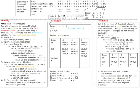
The central part of our approach is the LookupDB which

stores the experience data Figure 1 (middle box). Each of the elements of the LookupDB stores, among other things, a condition (cond), a step prediction, and a probability (P). This describes the probability (P) that the next step (prediction) will be started, given the occurrence of the step sequence cond. For example: An element of LookupDB can store the condition 1→2→3. When the steps 1→2→3 are observed, the probability that step 1 will be started is 0,9. Further, for each element in the condition sequence a set of relevant context probabilities are stored. Those are these contexts which were observed in the past.

For prediction (see Figure 1, right) of the next step all relevant elements of LookupDB are taken and for each of these elements an “actual probability” is calculated. Here, our approach considers the learned context relevance in LookupDB and the actual observed contexts in the corresponding window.

After prediction and after observation our algorithm learns this observation by updating the conditional probabilities and context relevance of all matching elements in the LookupDB (see Figure 1, left). In the following out approach is specified in a more detailed way.

First, let us define some relevant elements of our meta model (see [17-19]):

[image:3.595.63.536.423.721.2]

(1) Let S be index set which represents the set of Steps (2) Let C be index set which represents the set of

Figure 1. Overview of the approach.

Step: 1 2 3 1 2 3 1 2 3 1 2 3 1 2 3 1 2 3 1 2 3 1? ExcutionContext (IN): 4 5 6 4 5 6 7 8 9 7 8 9 4 5 6 7 8 9 4 5 6 4 ? ExecutionContext (OUT): 3 3 3 4 4 4 3 3 3 4 4 4 5 5 5 6 5 6 4 4 3 4 Kontext x: ...

Kontext y: ... ....

LookupDB Learning

After each observation:

For all elements in LookupDB which condition (Cond) matches to thelast observed steps(without last step – this will be learned) and thePrediction

matches to thelast observed step: 1. Update P:

P=alpha*P+(1-alpha) (see [22]) 2. Update Context relevance:

For each Index i:

For each line j (e.g. IN, OUT, …): let a be theactual context

observationin [i,j] update context relevance

K[a]=#observed a‘s in [i,j] / #observed contexts in [i,j] (this is the probability of a) 3. Update Context prediction:

Let c be the execution context to learn (IN of the last observed step).

Let l be a list of elements [Index:x,line] where c is observed in actual context observation

For all l: Update w: w=alpha*w+(1-alpha) 4. If last prediction was correct:

Add new elements to LookupDB (see [23] for the algorithm)

Prediction

Let L be a list of (copied) elements of LookupDB whichCond matches to the last observed steps (L contains copies of LookupDB – changes do not modify LookupDB)

For all l ∈L: 1. For each Index i:

For each line j (e.g. IN, OUT): let x be theactual context

observationin [i,j] delete all K[y] in the

Context relevance with y!=x in [i,j], e.g.:

2. Calcutales overall context relevance:

ocr=arithmetic mean of all K[*] in the Context relevance of l 3. Calculate P_actual = P * ocr Predict the l with the highest P_actual.

-2 K4=0,6 K4=0,5 …

-1 K5=0,3 K4=0,4 …

0 K6=0,3 K4=0,5 … Index

IN OUT … Index: -2 -1 0 IN: 4 5 6 OUT: 4 4 3 e.g. i=-2, j=IN: actual context

observationin [i,j] c = 4

Index: -2 -1 0

Cond : 1 2 3 Prediction: 1

P = 0,9

Context relevance:

Context prediction: [Index:0,IN] w = 0,9 [Index:0,OUT] w = 0,2 [Index:0,Kontext x] w = 0,2 [Index:1,IN] w = … …

-2 K4=0,6 K7=0,5 K3=0,8 K4=0,5 K6=0,1

…

-1 K5=0,3 K8=0,5 K3=0,1 K4=0,4 K5=0,2

… 0 K6=0,3 K9=0,7 K3=0,8 K4=0,5 K5=0,3 K6=0,2 … Index

IN OUT

Kontext x:

(4)

Contexts

(3) Let CC be index set which represents the set of Context Classifications.

To address the past observed steps we need an index set I:

(4) Let I be index set [ n,− …, 0].

The function observation returns the observed step at the index i, where i = 0 means the last observation, i = -1 the last but one observation, et cetera (see Figure 1 top right):

(5) observations:=DEF I→S

Furthermore, we need a function which returns the observed context at index i and at the Context Classification cc:

(6) observation2 :=_DEF

(

I CC×

)

→C

In the example in Figure 1, observation 2(0,IN) returns 6.

4.3. LookupDB

We define our LookupDB:

(7) Let LOOKUPDB:=DEF {0,1, 2, }… be Index Set Each element of LOOKUPDB represents an element of the LookupDB. Every element of our LookupDB has a condition cond. We define

(8) COND:=DEF{LOOKUPDB I× ×S}

COND is the set of all step sequences of elements of the LookupDB. For example: The following elements exist for the LookupDB element shown in Figure 1: (69,−2,1), (69,−1,0), and (69,0,3) where 69 is the ID of the shown LookupDB element. Let ldb∈LOOKUPDB;

, ldb i

cond describes the step of ldbat position i. (9) LENCOND:=DEF {LOOKUPDB×}

Is the set that describes the length of the condition de-fined in (8). The following element exists for the Loo-kupDB element described above: (69,3). The condition length is 3. Let ldb∈LOOKUPDB; lenCondldb de-scribes the condition length of ldb.

The set PREDICTION describes the predicted step of the element of the LookupDB:

(10) PREDICTION:=DEF{LOOKUPDB S× }.

(11) P:=_DEF {LOOKUPDB→

[ ]

0,1 } defines the probability of the element of the LookupDB that the predicted step occurs. For the element in Figure 1(69,1)

PREDICTION

∈ and (69, 0.9)∈P. For easy handling

ldb

p describes the probability of the LookupDB element ldb. Theset CONTEXTWEIGHT describes a weight for each context classification (Figure 1: the lines of the table, e.g. IN, OUT), index (Figure 1: rows of the table) and context (number in the fields of the table) for each element of the LookupDB:

(12)

{ }

CONTEXTWEIGHT

LOOKUPDB CC I C

∈ × × × × ×_{ }

The following elements describe the example in Fig- ure 1 at index 1, CC=IN:

(69,IN, 1,− K5, 3,10)∈CONTEXTWEIGHT; (3/10) defines the probability that the context K5 at position IN

and index-1 is relevant.

Now, we define a function that returns 1 if a specified entry of LookupDB corresponds to the last observed steps:

(1) match:=_DEF

(

LOOKUPDB×

) { }

→ 0,1

(

)

(

)

[

]

, , 1 if

: for all , 0

0 otherwise

ldb q s

ldb

match ldb offset

cond observation q offset

q lenCond

 = −



= ∈ −

 

Anymore, we define the following function that finds a specific element from the set CONTEXTWEIGHT:

(2) getCW: DEF LOOKUPDB CC I C CONTEXTWEIGHT

= × × ×

→

(

, , ,

)

:

getCW ldb cc i c =cw with

cw∈CONTEXTWEIGHT and

, ,

cw cw cw cw

id =ldb cc =cc i =i and c =c

4.4. Prediction

For prediction we define the following functions: (3) getAMC:=DEF {

(

I CC C× × ×

[ ]

0,1 }

)

→

[ ]

0,1

(

{( , , , )} :

)

with : arithmetic mean of all ( is threshold)

getAMC i cc c w amc amc

w θ θ

= =

> .

(4) f :=_DEF LOOKUPDB→{

(

I CC C× × ×[0,1] }

)

( ) (

{

)

}

[

]

(

)

(

)

: , , , with , 0 and

: 2 , for all and and

: / ( , ) : , , ,

ldb

f ldb i cc c w i lenCond c

observation i cc i cc w

x y with x y getCW ldb cc i c

= ∈ −

=

= =

The function f takes an entry of LOOKUPDB and returns a set of elements (index,cc,c,w). w corresponds to the context weight of ldb for each index i and cc in ldb

and for the corresponding c found in the observation. The function getAMC takes a set of elements ( in-dex,cc,c,w)and returns the arithmetic mean of all w. ge-tAMC(f(ldb))returns a “parameter” that the element of the LookupDB (and the learned context weights inside) cor-responds to the observed contexts.

The function getActualP takes an entry of LOO-KUPDB and calculates an actual P weight dependent on

ldb and the actual observation (this weight is used to se-lect the best entry of LOOKUPDB for prediction):

(5) getActualP:=_DEF LOOKUPDB→

[ ]

0,1

( )

:

(

( )

)

ldb}

getActualP ldb =getAMC f ldb ∗p

(5)

step:

(6) makeprediction:=DEF Pow LOOKUPDB( )→S ( ) : )

makeprediction ldb =s with

( )

: for maximal

s = prediction ldb getActualP ldb

To predict the next step we call the function make pre-diction with a set of all elements ldb of LookupDB with

match(ldb,0) = 1.

4.5. Learning

To update the LookupDB, the following steps are done (note: observations(0) is the step a prediction we made and we want to learn):

If there exists no ldb∈LOOKUPDB with (ldb,1)∈LENCOND and

((ldb, 0),observation( 1))− ∈COND and

(ldb observation, s(0))∈PREDICTION a new entry is added to the LookupDB (the entry with the shortest cond):

(19)

: { } { }

{ } { } { }

{ } { }

{ } { } { }

DEF

addEntry LOOKUPDB COND

LENCOND PREDICTION P

LOOKUPDB COND

= ×

× × ×

→ ×

× × ×

0 0, 0 0 0

1 1 1 1 1

( , , , ) :

( , , , ,

addEntry ldb cond lc pre p

ldb cond lc pre p

=

with:

• 1 0 1 0 1 0

1 0 1 0

\ , \ , \

, \ , \ )

ldb ldb cond cond lc lc

pre pre p p

= ∅ = ∅ =

∅ = ∅ = ∅

• 0 1 0 1 0

1 0 1 0 1

1 , 1 ,

1 , 1 , 1

ldb ldb cond cond lc

lc pre pre p p

+ = + = +

= + = + =

• n∉ldb₀andn∈ldb₁

•

0 1

( , 0, ( 1))

and (( , 0), ( 1))

n observation

cond n observation cond

− ∉

− ∈ • ( ,1)n ∉lc₀and ( ,1)n ∈lc₁

•

0 1

( , (0))

and( , (0))

s

s n observation

pre n observation pre

∉ ∈

• ( ,1n −α)∉p₀and( ,1n −α)∈p₁

Let LDB⊆LOOKUPDB:

{ |

LDB= ldb∈LOOKUPDB

(

)

( )

,1

1 ( , _s 0 ) }.

match ldb

and l observation PREDICTION

= ∈

For each element ldb∈LDB the following steps are done:

(20) updateP:=_DEF

{ }

P ×LOOKUPDB→{ }with :P

(

)

(

)

(

)

(

)

(

0 1

)

0

1 1 0

, : , , ,

, * 1 andp \ {(ldb, pp)}

updateP p ldb p with ldb pp p ldb pp

p and ldbα pp α p

= ∈ ∉

+ − ∈ =

1{( , * (1 ))}

p elbα pp+ −α (see [15])

(21)

{

}

: _DEF

updateContextweight = CONTEXTWEIGHT

{ }

LOOKUPDB CONTEXTWEIGHT

× →

(

0,

)

: 1with updateContextweight cw el =cw

• For all

(

ldb cc i c x y, , , , ,

)

∈cw0 with

1 ( , , , , , )

ldb≠el⇒ ldb cc i c x y ∈cw

• For all

(

ldb cc i c x y, , , , ,

)

∈cw0with ldb=el and

(

) (

)

1 1

2 , , , , , , and ( , , , , 1, 1)

c observation i cc ldb cc i c x y

cw ldb cc i c x y cw

= ⇒ ∈

+ + ∈

• For all (ldb cc i c x y, , , , , )∈cw0 with ldb=eland

( ) (

)

1 1

, , , , , and ( , , , , , 1)

s

c observation i ldb cc i c x y

cw ldb cc i c x y cw

≠ ⇒ ∉

+ ∈

This function updates the probabilities of the context information in ldb.

If the last prediction was correct new entries are added to the LookupDB according to the work of Jacobs et al.

[16]. Let Q⊆LOOKUPDB be a subset of LOO-KUPDB with:

(22) Q:=DEF{ldb∈LOOKUPDB cond| q i,

(

1 for all

)

, 0 }

s

q

observation i i

lenCond

= −

 

∈  

Let L⊆LOOKUPDB be subset of LOOKUPDB

with:

(23) L:=_DEF{ldb∈LOOKUPDB cond| _{l i}_,

( )

[

]

for all , 0 }

s

ldb

observation i i

lenCond

= ∈

Let ll be the element of L with the longest lenCond and

P(ll)>0. The function update LOOKUPDB is defined as: (7)

{

}

{ }

{

} {

} { }

:

{ }) ({ } { }

{ } { } {

}) (

} {

DEF

updateLOOKUPDB LOOKUPDB Q ll

COND LENCOND PREDICTION P

CONTEXTWEIGHT LOOKUPDB COND

CONTEXTWEIGHT

= × × ×

× × × ×

→ × ×

× × ×

(

0, , , 0, 0, 0, 0, 0

)

:

updateLOOKUPDB LDB q l c lc pre p cw =

(

LDB c lc pre p cw1, ,1 1, 1, 1, 1

)

with (see [16]):

• 0

1 0 1

{0,1, , } and {0,1, , , } | | | | | |

n LDB n m

LDB with LDB q LDB

… ∈ … … ∈

+ =

Let ldiff be LDB₁\LDB₀. For all there is an in with :

qq∈q ldiffel lediff

•

0 1

1

(( , ), ) and(( , 1), )

for all and ; and : (( , 0), (0))

q i s c ldiffel i s

c i s ldiffel oberservation

c

∈ − ∈

∈

• ( , )q l ∈lc₀and (ldiffel l, + ∈1) lc₁

• ( , )q s ∈pre₀and (ldiffel s, )∈pre₁for alls

• ( , )q p ∈p₀and( , 2)ll p ∈p₀and(ldiffel p, 2)∈p₁

(6)

and “extending” the corresponding conditions by adding the observation (see [16] for detail).

5. Evaluation

5.1. Synthetical Process

For the evaluation of the approach described in Section 4 we derived a synthetic project scenario. In this scenario the requirements of the system are existent. The goal is to develop an architecture (components, classes) and a corresponding implementation. The process description con- sists of 4 steps: 1) Identify component, 2) Map requirement to Component, 3) Specify component (refine requirement), 4) Implement component.

In the system two types of components exist: a) Com- plex/hardware related components. Here, the engineer has a prototypical method to develop the component (steps 2 - 4 are executed sequentially). b) Components which classes have a high coupling. Here, the engineer has a broad design method (step1; all steps 2; all steps 3; all steps 4).

For evaluation three sequences of steps (with corresponding contexts) were build: i) Development of components only of the type a), ii) Development of components only of the type b), and iii) random mix of a) and b).

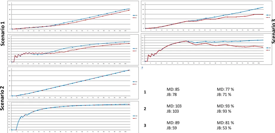
Our approach is compared with the algorithm from Jacobs/Blockeel [16] which is the underlying sequence prediction technique of our approach. The results are shown in Figure 2. This figure contains two graphs for each scenario: The first (top) describes the total number of correct predictions and the second describes the per- centage distribution of correct prediction after each step

(horizontal axis). The Jacobs Blockeel(JB) approach is shown in red color and our approach (MD) is shown in blue color.

In all scenarios our approach predicts equal to or better than the Jacobs Blockeel algorithm. Remarkable is that in scenario 3 (the “real world” scenario) our approach predicts the steps substantially better than the JB approach. After 2/3 of all steps our algorithm predicts always correctly. On the other hand the algorithm of JB “drifts” to 53% correct predictions. 81% of correct predictions in scenario 3 might be an indication that our approach is more applicable.

5.2. Real Project Process

In addition to the synthetical evaluation (described in section V.A) we evaluated our approach with real project data from anindustrial enterprise. Are there differences between these two evaluations? In the synthetical evaluation we described a process description using the description language presented in Section 3. This is a rule based language which is flexibly executable for the engineer. On this basis, we derived three test data sets and evaluated our approach with these data. The evaluation of the industrial case study is based on real project data with 5.600 individual development steps. The underlying process description language of the industrial case study was a net based language. Therefore, the process description (and the enacted process) is more stringent than our process used for evaluation in section V.A.

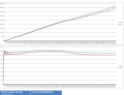
[image:6.595.67.529.492.715.2]

Like in the synthetically evaluation our approach is compared with the approach of Jacobs/Blockeel. The results are shown in Figure 3. Again, there are two cate-

Figure 2. Results synthetic scenario. 0

20 40 60 80 100

REFERENCES

[1] L. Northrop, P. Feiler, R. P. Gabriel, J. Goodenough, R. Linger, T. Longstaff, R. Kazman, M. Klein, D. Schmidt, K. Sullivan and K. Wallnau, “Ultra-Large-Scale Systems —The Software Challenge of the Future,” Software En- gineering Institute, Carnegie Mellon, Tech. Rep., 2006. http://www.sei.cmu.edu/uls/downloads.html
[2] A. W. Brown and J. A. McDermid, “The Art and Science of Software Architecture,” In: F. Oquendo, Ed., ECSA, Ser. Lecture Notes in Computer Science, Vol. 4758, Springer, 2007, pp. 237-256.
[3] B. Boehm, “Some Future Trends and Implications of Sys- tem and Software Engineering Processes,” Wiley InterS-cience, 2006.
[4] D. Rombach, “Integrated Software Process and Product Lines, Unifying the Software Process Spectrum,” 2006.
[5] M. Kabbaj, R. Lbath and B. Coulette, “A Deviation Ma- nagement System for Handling Software Process Enact- ment Evolution,” Making Globally Distributed Software Development a Success Story, 2008, pp. 186-197.
[6] K. Mohammed, L. Redouane and C. Bernard, “A Devia- tion-Tolerant Approach to Software Process Evolution,” Ninth International Workshop on Principles of Software Evolution in Conjunction with the 6th ESEC/FSE Joint Meeting, 2007, pp. 75-78.
[7] D. Jean-Claude, K. Badara and W. David, “The Human Dimension of the Software Process. In: Software Process:
Principles, Methodology, and Technology, Lecture Notes in Computer Science,” Bd. 1500, Springer US, 1999, pp. 165-199.
[8] T. DeMarco and T. Lister, “Peopleware, Productive Pro- jects and Teams, Second Edition Featuring Eight All- New Chapters,” Dorset House Publishing Corporation, 1999.
[9] K. Z. Zamli, “Process Modeling Languages: A Literature Review,” Dez-2001.
http://myais.fsktm.um.edu.my/278/
[10] S. T. Acuna, “Software Process Modelling.”
[11] P. Armenise, S. Bandinelli, C. Ghezzi und A. Morzenti, “A Survey and Assessment of Software Process Repre- sentation Formalisms,” International Journal of Software Engineering and Knowledge Engineering, Bd. 3, 1993, pp.
401-
[12] M. I. Kellner, “Representation Formalisms for Software Process Modeling,” Proceedings of the 4th International Software Process Workshop on Representing and Enact- ing the Software Process, Devon, United Kingdom, 1988,
pp. 93-96
[13] P. H. Feiler und W. S. Humphrey, “Software Process De- velopment and Enactment: Concepts and Definitions,” Software Process, 1993, Second International Conference on the Continuous Software Process Improvement, 1993, pp. 28-40.
[14] M. Hartmann und D. Schreiber, “Prediction Algorithms for User Actions,” Proceedings of Lernen Wissen Adap- tion, ABIS, 2007, pp. 349-354.
[15] B. D. Davison und H. Hirsh, “Predicting Sequences of User Actions,” Notes of the AAAI/ICML 1998 Workshop on Predicting the Future: AI Approaches to Time-Series Analysis, 1998.
[16] N. Jacobs und H. Blockeel, “Sequence Prediction with Mix- ed Order Markov Chains,” Proceedings of the Belgian/ Dutch Conference on Artificial Intelligence, 2002. [17] M. Deynet, “User-Centric Process Descriptions,” Pro-
ceedings of the 3rd International Conference on Software Technology and Engineering, Kuala Lumpur, Malaysia, 2011, pp. 209-214.
[18] M. Deynet, “Kontextsensitiv Lernende Sequenzvorher- sage zur Erfahrungsbasierten Unterstützung bei der Soft- wareprozessausführung,” Dr. Hut, 2013.