in high-dimensional biological data
A thesis presented for the degree of Doctor of Philosophy of Imperial College
by
Zi Wang
Department of Mathematics Imperial College
180 Queen’s Gate, London SW7 2AZ
2
I certify that this thesis, and the research to which it refers, are the product of my own work, and that any ideas or quotations from the work of other people, published or otherwise, are fully acknowledged in accordance with the standard referencing practices of the discipline.
Copyright
Copyright in text of this thesis rests with the Author. Copies (by any process) either in full, or of extracts, may be madeonlyin accordance with instructions given by the Author and lodged in the doctorate thesis archive of the college central library. Details may be obtained from the Librarian. This page must form part of any such copies made. Further copies (by any process) of copies made in accordance with such instructions may not be made without the permission (in writing) of the Author.
The ownership of any intellectual property rights which may be described in this thesis is vested in Imperial College, subject to any prior agreement to the contrary, and may not be made available for use by third parties without the written permission of the University, which will prescribe the terms and conditions of any such agreement. Further information on the conditions under which disclosures and exploitation may take place is available from the Imperial College registry.
4
Abstract
Recent advances in technology have made it possible and affordable to collect biological data of unprecedented size and complexity. While analysing such data, traditional statis-tical methods and machine learning algorithms suffer from the curse of dimensionality. Parsimonious models, which may refer to parsimony in model structure and/or model pa-rameters, have been shown to improve both biological interpretability of the model and the generalisability to new data.
In this thesis we are concerned with model selection in both supervised and unsuper-vised learning tasks. For superunsuper-vised learnings, we propose a new penalty called graph-guided group lasso (GGGL) and employ this penalty in penalised linear regressions. GGGL is able to integrate prior structured information with data mining, where variables sharing similar biological functions are collected into groups and the pairwise relatedness between groups are organised into a network. Such prior information will guide the selection of variables that are predictive to a univariate response, so that the model selects variable groups that are close in the network and important variables within the selected groups. We then generalise the idea of incorporating network-structured prior knowledge to associ-ation studies consisting of multivariate predictors and multivariate responses and propose the network-driven sparse reduced-rank regression (NsRRR). In NsRRR, pairwise relat-edness between predictors and between responses are represented by two networks, and the model identifies associations between a subnetwork of predictors and a subnetwork of responses such that both subnetworks tend to be connected. For unsupervised learning, we are concerned with a multi-view learning task in which we compare the variance of high-dimensional biological features collected from multiple sources which are referred as “views”. We propose the sparse multi-view matrix factorisation (sMVMF) which is
6
parsimonious in both model structure and model parameters. sMVMF can identify latent factors that regulate variability shared across all views and the variability which is charac-teristic to a specific view, respectively. For each novel method, we also present simulation studies and an application on real biological data to illustrate variable selection and model interpretability perspectives.
Acknowledgements
Mediocre teachers tell, good teachers explain, superior teachers demonstrate, exceptional teachers inspire (William Ward). This work could not have been achieved without the valuable motivation and assistance from Prof. Giovanni Montana, a good, superior, and ex-ceptional supervisor. I would also like to thank Dr. Edward Curry, Dr. Michelle Krishnan, Peter Nash, Dr. Anand Pandit, and Dr. Wei Yuan, who have introduced me to various areas in computational biology and neuroimaging science, and with whom I have collaborated on several interesting projects during my PhD studies. I am very grateful to the Biological Research Council for their generous support (DCIM-P31665) to my research.
The three and a half years of life as a PhD student has been fruitful and more impor-tantly (and perhaps surprisingly) exciting and memorable because of the following people whom I feel deeply indebted to: My parents Xueyan Wang and Xiaozhong Wang for their unconditional love; Two of my dearest mentors Anne Scott and Dr. Brian Brooks, who have been my best listeners and most trustworthy advisors for the past ten years; Prof. Roderich Swanston, whose lunchtime lectures on classical music and western civilisation at Imperial College were the most amazing lectures I have ever attended; Dr. Sehun Chang, who guided me to the grand palace of classical music and fine art and developed my fa-natic enthusiasm (of spending) on them; My office mates Dr. Ai Chung, Zhana Kuncheva, Dr. Rudra Poudel, and Petros Ypsilantis, for the constructive academic discussions they offered, and for their indifference to coffee (except for Petros) and yet their obsession to coffee breaks which helped me retain my sanity when typing up this thesis; My landlords Graham and Miranda Broomfield for providing comfortable and hearty accommodation and the daily three-course gourmet dinners, which always got me fully charged for the works to do the next day; All my students, whom I taught at Imperial College, King’s
Col-8
lege London, and on private occasions, for giving me the chance to acquire immense self esteem from teaching and being appreciated; And last but not the least, my girlfriend, who did not emerge during this period.
Table of contents
Abstract 5
List of Publications 12
1 Introduction 14
1.1 Challenges in pattern recognition in biological data . . . 14
1.2 Introduction to regularisation methods . . . 16
1.3 Summary of contributions . . . 18
1.3.1 Graph-guided group lasso . . . 18
1.3.2 Network-driven sparse reduced-rank regression . . . 18
1.3.3 Sparse multi-view matrix factorisation . . . 19
2 The graph-guided group lasso 20 2.1 Introduction to genome-wide association studies. . . 20
2.2 Introduction to unstructured penalties . . . 26
2.3 Introduction to structured penalties . . . 36
2.3.1 Group-structured penalties . . . 36
2.3.2 Graph-structured penalties . . . 42
2.4 Bayesian methods . . . 47
2.5 The graph-guided group lasso model . . . 48
2.6 Properties . . . 52
2.6.1 GGGL-1: smoothing effect. . . 52
2.6.2 GGGL-2: smoothing effect. . . 55
2.7 Serial block coordinate descent algorithm . . . 58
2.7.1 Serial algorithm for GGGL-1. . . 58
2.7.2 Serial algorithm for GGGL-2. . . 61
2.8 Parallel coordinate descent algorithm . . . 62
2.8.1 Introduction to parallel computing . . . 62
2.8.2 Parallel coordinate descent algorithm . . . 63
2.9 Parameter tuning . . . 67
2.9.1 Stability selection. . . 69
10
2.10 Simulation studies. . . 71
2.11 Application: pathway-based imaging genomics in preterm infants . . . 75
2.11.1 Introduction . . . 75
2.11.2 Data preparation . . . 76
2.11.3 Results . . . 77
2.12 Discussion and Conclusion . . . 81
3 Network-driven sparse reduced-rank regression 84 3.1 Introduction to DNA methylation and gene expression association studies . 84 3.2 The reduced-rank regression . . . 88
3.3 The sparse reduced-rank regression. . . 91
3.4 Network-driven sparse reduced-rank regression . . . 93
3.4.1 Problem formulation . . . 93
3.4.2 Model . . . 93
3.5 Estimation algorithm . . . 96
3.5.1 Parameter tuning procedures . . . 99
3.6 Simulation studies. . . 99
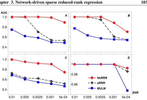
3.7 An application to ovarian cancer . . . 103
3.7.1 Introduction. . . 103
3.7.2 Material and method . . . 104
3.7.3 Results . . . 105
3.8 Connection with other models . . . 120
3.8.1 Connections with latent variable models . . . 120
3.8.2 Connections with multi-task regressions . . . 125
3.8.3 Bayesian models . . . 131
3.9 Discussion and conclusion . . . 131
3.10 Appendix . . . 134
4 Sparse multi-view matrix factorisation 137 4.1 Motivation and background . . . 137
4.2 A survey on unsupervised multi-view learning . . . 140
4.2.1 Co-training algorithms . . . 140
4.2.2 Manifold alignment. . . 141
4.2.3 Subspace learning algorithms . . . 145
4.3 Sparse multi-view matrix factorisation . . . 149
4.3.1 Multi-view matrix factorisation model . . . 150
4.3.2 Sparsity constraints and estimation. . . 153
4.3.3 Parameter selection . . . 157
4.4 Illustration with simulated data . . . 159
4.4.1 Simulation setting . . . 159
4.4.2 Simulation results . . . 162
4.5.1 Data preparation . . . 167
4.5.2 Experimental results . . . 168
4.5.3 Anad hocrobustness study on the choice of(d, r) . . . 180
4.6 Relation to other relevant models . . . 182
4.6.1 JIVE . . . 182
4.6.2 HO-GSVD . . . 184
4.7 Conclusion and Discussion . . . 185
4.8 Appendix . . . 188
5 Conclusions and future works 191 5.1 Conclusions . . . 191
5.2 Future works . . . 194
A 197
12
List of Publications
1. A. Pandit, E. Robinson, P. Aljabar, G. Ball, I. Gousias, Z. Wang, J. Hajnal, D. Rueck-ert, S. Counsell, G. Montana and A. Edwards. Whole-brain mapping of structural connectivity in infants reveals altered connection strength associated with growth and preterm birth. Cerebral Cortex, 10.1093.bht086. 2013.
This can be downloaded from:
http://cercor.oxfordjournals.org/content/early/2013/03/31/ cercor.bht086.full
2. Z. Wang, E. Curry and G. Montana. Network-guided regression for detecting associ-ations between DNA methylation and gene expression. Bioinformatics, 30(19):2693-2701, 2014.
This can be downloaded from:
http://bioinformatics.oxfordjournals.org/content/30/19/2693. full
3. Z. Wang and G. Montana. The graph-guided group lasso for genome-wide associ-ation studies. In “Regularization, Optimization, Kernels, and Support Vector Ma-chines”. J. Suykens, M. Signoretto and A. Argyriou (editors) Chapman & Hall/CRC Machine Learning & Pattern Recognition, pp.131-158, 2014.
4. Z. Wang, W. Yuan and G. Montana. Sparse multi-view matrix factorisation: a mul-tivariate approach to multiple tissue comparison. Accepted by Bioinformatics, to appear.
5. M. Krishnan, Z. Wang, M. Silver, J. Boardman, G. Ball, S. Counsell, A. Walley, G. Montana and D. Edwards. Lipid pathways mediate genetic susceptibility to brain injury in preterm infants. Submitted toHuman Brain Mapping.
14
Chapter 1
Introduction
1.1
Challenges in pattern recognition in biological data
The last two decades have witnessed a large amount of various biological data such as single nucleotide polymorphisms (SNPs), genome-wide microarray gene expressions and DNA methylations being produced, which provided a wealth of information to understand the complex biological mechanisms and their consequences. Statistical modeling and ma-chine learning are among the main tools to resolve such learning tasks. For instance, one may carry out an association study between SNPs data and gene expression data to iden-tify genetic variants that affect gene regulation. This type of study, referred as expression quantitative trait loci (eQTL) mapping, can reveal substantial heritable variation in gene expression within and between populations [Gilad et al.,2008]. For another example, one may compare global mRNA expression data collected from multiple organisms at multi-ple time points during the cell-cycle, hoping to reveal common and distinctive cell-cycle mRNA expression oscillation patterns among and within the disparate organisms [ Ponna-palli et al., 2011]. On one hand, statistical models and machine learning algorithms have generated and led to numerous biological discoveries; on the other hand, they have been constantly challenged by the ever increasing dimensionality, complexity, and variety of biological data.
The first challenge to existing statistical models and machine learning algorithms arises from the high dimensionality of the data. By high dimensional data we refer to the case
where the number of subjects is much smaller than the number of measurements (vari-ables). This problem makes it challenging to estimate the parameters of a model. For instance, when we fit a linear regression model to a high dimensional dataset with a uni-variate response, the design matrix would be rank deficit and the linear coefficients could not be computed in the normal way. Secondly, many high dimensional data are very noisy, thus for models which are sensitive to noise and uncertainty, model interpretation and pre-diction performance may suffer from overfitting.
The second challenge is that high dimensional biological data often have many re-dundant features and only a small subset of the features are relevant to the desired study. Therefore, parsimony is necessary to data mining and the understanding of the underlying biological processes. Here, the meaning of parsimony lies in two aspects: parsimonious structure and/or sparse model parameters. In unsupervised learning, the majority amount of non-random variability within a dataset may be driven by a few latent factors, in which case dimensionality reduction techniques will capture the intrinsic variability of the dataset while reducing the complexity of the model. In supervised learning, associations between multivariate predictors and multivariate responses may be driven by a few latent factors, in which case models with parsimonious structure would be more appropriate and better at revealing the true biological interactions. However, since biological data often consist of thousands and even up to a few millions of variables, a model with parsimonious structure in which each latent factor regulates all variables is still difficult to interpret and may well result in model overfitting. Imposing sparsity in model parameters can enable us to identify the subset of features that are truly relevant to the desired study, which offers more biolog-ical insights and improves the generalisability to new data [Tibshirani, 1996, Jongeneel et al.,2005].
The third challenge arises from the variety of data that are available which may be incorporated to improve the interpretability of the model. For example in an association study where our interest lies in identifying predictive SNPs to a disease-related trait, apply-ing hypothesis testapply-ing or some simple algorithms may only extract a few SNPs randomly located in the genome each carrying a strong effect, but fail to identify the vast amount of genetic variants each carrying a moderate or weak effect yet jointly participating in some biological process and having a large influence on the trait. A remedy to improve variable
1.2 Introduction to regularisation methods 16
selection results would involve incorporating existing biological knowledge and promoting the selection of SNPs belonging to genes which are known to participate in a biological process that are relevant to the study. The success of this strategy will depend on select-ing the relevant information to be integrated with the statistical model or machine learnselect-ing algorithms, and how the additional information is integrated with the datasets to guide vari-able selection in deriving biologically plausible models [Tibshirani et al.,2005,Wang et al.,
2010,Silver and Montana,2012].
In this thesis, we shall present three novel models motivated by three studies involving high dimensional biological datasets. A common technique called “regularisation” will be used to address the challenges posed by such data. In Section 1.2 we briefly introduce regularisation methods, and we introduce the biological problems and summarise our con-tributions in Section1.3.
1.2
Introduction to regularisation methods
Many statistical models and machine learning algorithms can be formulated as an optimi-sation problem in which a loss functionfis minimised. Examples offinclude the squared loss for regression models and the hinge loss and logistic loss for classification. We con-sider a regression model in which observations on ppredictor variables collected from n
samples are arranged in ann×pmatrixX, and the univariate response is denoted by n -dimensional vector y. In statistical modeling, the association between predictors and the univariate response is typically quantified by ap-dimensional vectorβ, whose estimate is obtained by minimising a function f: Rp → R. We assumef is smooth and Lipschitz continuous. In regression settings,f is typically taken as the squared loss and the estimates ofβ can be obtained by solving:
minimise: f(β) =ky−Xβk2 2
where k.k2 refers to the `2-norm. Estimated coefficients denoted by βˆcan be explicitly obtained by:
ˆ
β = (XTX)−1XTy (1.1)
where the superscript T denotes matrix transpose, provided that the inverse of (XTX) exists. However, in the context of high dimensional data wheren << p,X does not have full column rank and that(XTX)−1does not exist. A remedy of this is to search the optimal
β that minimisesf within a constraint region defined byΩ(β)≤ 0, where the functionΩ: Rp →R+∪ {0}is referred as the “penalty function”. Apart from making the computations feasible, such a constraint may also impose a desired pattern to the estimatesβˆ, obtained by solving the constrained optimisation problem:
minimise: f(β)
subject to: Ω(β)≤0 (1.2)
Under mild conditions [di Pillo and Grippo,1989,Boyd and Vandenberghe,2004], solution to (1.2) is equivalent to that of:
minimise: f(β) +λΩ(β) (1.3)
whereλis a non-negative regularisation parameter which controls the weight of the penalty
Ω. Statistical models and machine learning algorithms which amount to optimising (1.3) are referred as regularisation methods.
For convenience of the discussion, we categorise penalties into “structured” and “un-structured” types. Structured penalties enforce or encourage a particular pattern on the estimated coefficients βˆbased on either prior knowledge or some measure of relatedness derived from the data. Therefore the solution to (1.3) depends on both the data and the structure the penalty imposes. Unstructured penalties may well enforce particular patterns on the solution such as sparsity, however, the solution is solely data-driven as no prior knowledge is considered by the model. A comprehensive survey unstructured and struc-tured penalties will be given in Section 2.2 and 2.3. A brief discussion of incorporating
1.3 Summary of contributions 18
prior information in Bayesian models is given in Section2.4where we also draw connec-tions with frequentist approaches (i.e. penalties).
1.3
Summary of contributions
1.3.1
Graph-guided group lasso
In Chapter2, we consider a linear regression problem with a univariate response, and pro-pose a new penalty called “graph-guided group lasso (GGGL)”. This work is motivated by genome-wide association studies (GWAs) in which we search for SNPs that are most predictive to a univariate trait. We firstly give a comprehensive review of classic and state-of-the-art penalties which can impose various patterns on model parameters. We then pro-pose the GGGL which can integrate prior biological information in the form of gene-SNP mapping and a gene network representing pairwise relatedness between the genes such that the model promotes selection of functionally related genes and important SNPs within such genes. We present a serial estimation algorithm which cyclically updates the coefficients of one group (gene) of variables (SNPs) at a time and a parallelised estimation algorithm implemented on graphics processing units (GPUs) which updates the coefficients of sev-eral groups of variables simultaneously in one step. We also give a new variable ranking algorithm which can determine the optimal weight of the prior information in relation to the loss function and rank the variables according to their importance in model. We report the results in simulation studies and our findings in an application of a GWA.
The GGGL methodology and simulation results were published inWang and Montana
[2014]. The GWAs application was included inKrishnan et al.[2015], collaborated with Michelle Krishnan and others. Peter Nash helped with the implementation of the paral-lelised estimation algorithm on GPUs.
1.3.2
Network-driven sparse reduced-rank regression
In chapter3, we generalise the linear regression problem in the previous chapter to allow multivariate responses. We extend the previous work of sparse reduced-rank regression (sRRR) [Vounou et al.,2010] to network-driven sparse reduced-rank regression (NsRRR)
which searches associations between multivariate predictors and multivariate responses while integrating prior information in the form of two networks describing the pairwise relatedness between the predictors and responses, respectively. This work is motivated by an association study in which we aim to identify a small subset of functionally related DNA methylations and a small subset of expression measurements corresponding to some func-tionally related genes which are strongly correlated. We present simulation results and our discoveries in an ovarian cancer study. We also include a technical discussion on the con-nections between reduced-rank regression, latent variable model, and multi-task regression, all of which can be applied to solve this type of problem.
The NsRRR methodology, simulation and application results were published in Wang et al.[2014]. The application was done in collaboration with Dr Edward Curry.
1.3.3
Sparse multi-view matrix factorisation
Chapter4deals with a multi-view learning problem in which we compare the same biolog-ical measurements obtained from more than two population groups or from more than two environment conditions. This work is motivated by analysing mRNA expression measure-ments collected from three tissue groups where our objective is to distinguish the variability among the subjects that is shared across all tissues from the variability that is characteris-tic to a specific tissue. We firstly present a review of existing methods for unsupervised multi-view learning where the task is to understand the common features (and possibly view-specific features too) across multiple representations of the same data objects referred as “views”. We then present the sparse multi-view matrix factorisation (sMVMF) model which seeks latent factors that drive the non-random variability shared across all tissues and specific to each tissue respectively and identifies important gene expressions for each latent factor. We apply sMVMF to simulated and real data from the TwinsUK cohort to demonstrate its performance.
The sMVMF methodology, simulation and application results were included in Wang et al.[2015], which has been accepted for publication. The application was done in collab-oration with Dr Wei Yuan.
20
Chapter 2
The graph-guided group lasso
2.1
Introduction to genome-wide association studies
Individual in a human population each has a unique set of traits, such as height, weight, skin/hair/eye colour, dialect, intelligence, and intestinal permeability. Traits which are di-rectly observable or measurable are called “phenotypic traits”, and some phenotypic traits, for instance intestinal permeability, may be indicators of disease status or quantitative mea-sures of disease risk or physical properties [Frazer et al., 2009]. While variation in traits such as dialect and perhaps weight amongst individuals may be caused or predominately affected by environmental factors, variation in other traits such as skin and eye colour is generally arisen from the difference in gene frequencies, which is referred as genetic vari-ation. Human genetic variation consists of many types, for instance, copy number varia-tion, insertion-deletion variavaria-tion, inversion variavaria-tion, and single-nucleotide polymorphism (SNP) which is the most common type [Frazer et al., 2009]. Each SNP represents a vari-ation in the genome where a single nucleotide - Adenine (A), Thymine (T), Cytosine (C), or Guanine (G) - differs between paired chromosomes. SNPs occur regularly at an average frequency of one in300nucleotides in a human DNA sequence. While most SNPs have no effect on disease development, some have been proved to have a causal effect on various diseases. The associations between genetic variations and human traits have traditionally been investigated through inheritance studies in families [Easton et al., 1993]. While this has proved useful for single gene disorders, associations identified with complex diseases
involving multiple genetic determinants are hard to reproduce [Altm¨uller et al., 2001]. In the last decade, the number of genome-wide association studies (GWAs) has increased im-mensely [Haines et al., 2005, Ku et al., 2010, Ripke et al., 2011, Cui et al., 2013]. GWAs search common genetic variants across the human genome in unrelated individuals that are associated with a trait. They have succeeded in identifying reproducible associations with thousands of human diseases and traits [Johnson and O’Donnell, 2009, Li et al., 2012b,
Leslie et al.,2014]. This work is motivated by a GWAs application in which we assume the genetic variants are SNPs, and we develop a statistical method to identify SNPs associated with a univariate trait. We refer the SNPs/genes having a non-random association with the trait as “associated SNPs/genes”, which are to be inferred.
GWAs typically consist of a case-control study design, in which the subjects are par-titioned into case and control groups, and hypothesis tests (e.g. based onχ2 statistic) are carried out for each SNP to examine if the allele frequencies are significantly altered be-tween the case and control groups [The Wellcome Trust Case Control Consortium, 2009,
Clarke et al.,2011]. An illustration of a case-control design of GWAs is given in Figure2.1. Some limitations of this approach include: substantial estimation biases and spurious asso-ciations due to violation of the assumptions in case-control design [Pearson and Manolio,
2008]; insufficient sample size in comparison to the number of variables - typically sample sizes vary between a few hundreds and a few thousands, whereas the number of SNPs to be investigated is about 1 million and may go beyond 10 millions [The Wellcome Trust Case Control Consortium, 2009, National Center for Biotechnology Information, 2014]; and multiple testing issues [Pearson and Manolio,2008].
2.1 Introduction to genome-wide association studies 22
Figure 2.1: An illustration of the work-flow in a case-control design of GWAs. Subjects are partitioned into case and control groups. For each SNP, a hypothesis test is performed to examine if allele frequencies are significantly different between the case and control groups.
measure-ment rather than a binary indicator. We assume that the SNPs have been genotyped and we denote the major allele by “A” and the minor allele by “a”, such that the genotypes can be expressed as one of “AA”, “Aa”, and “aa”. We further assume a linear regression model with additive genetic effects [Stranger et al., 2007], such that the predictors take values
0, 1, or2 which represent the number of minor alleles at each locus, and the strength of associations can be quantified by the coefficients of the linear regression model. When the number of subjects is greater than the number of SNPs, the coefficients can be estimated by minimising the empirical loss function (the squared loss). A t-test can then be performed on the linear coefficient to evaluate whether the genetic effect is significant [Uda et al.,
2008]. However, in GWAs, the number of SNPs typically greatly exceeds the number of subjects, which raises computational issues in coefficients estimation. Many regularised methods have been proposed to tackle this problem, which involve adding a penalty term of the coefficient vector to the objective function being minimised [Signoretto et al.,2009,
Ojeda et al., 2010, Chen et al., 2010a, Hoffman et al., 2013]. Taking the `1 norm of the coefficient vector as the penalty term, amongst others, some entries in the estimated co-efficients are set to zero and a set of important SNPs can be automatically selected which correspond to the non-zero entries in the estimated coefficient vector [Tibshirani,1996].
In GWAs and other applications, there appears to be two trends in the recent develop-ment of penalised linear regression models. The first is developing fast computation algo-rithms that can be applied to “big data” problems [Richt´arik and Tak´aˇc, 2013a,b], where the sample size is as large as 200,000 or more [ICBP, 2011] and the number of predic-tors is comparable or much larger than the sample size; the second trend is developing new penalties to impose biologically informed sparsity patterns. The motivation is that the variability in disease related traits often arises from the joint contribution from multiple loci within a gene and the joint action of genes within a pathway [Luo et al., 2010,Silver et al.,2013]. Although some genetic variants may only facilitate a moderate or weak effect on the trait individually, their joint effect could be influential. Unfortunately, the set of SNPs extracted by purely data-driven methods often account for only a small proportion of the genetic variants associated with the trait, which may provide very limited insight into the biological mechanisms underpinning the complex disease [Manolio et al., 2009]. One promising approach involves incorporating prior biological information on the functional
2.1 Introduction to genome-wide association studies 24
relations between the genetic variants to guide the selection of associated predictors. The hope is that the penalty function acting on this information will encourage the selection of co-functioning genetic variants and hence producing a set of important predictors explana-tory of the variability in the trait as well as biologically plausible [Tibshirani et al., 2005,
Wang et al.,2010,Silver and Montana,2012].
Prior information on the relatedness between variables, which we shall refer to as “structured knowledge” [Bach et al.,2012], can be organised in many ways. In the context of genetics studies, one way to organise the structured knowledge regarding co-functioning SNPs and genes is partitioning the candidate SNPs into non-overlapping groups according to the gene-SNP mapping, where each group corresponds to a set of SNPs that constitute a gene or a pathway. Using the group lasso penalty [Yuan and Lin, 2006], the model can identify a set of important genes or pathways which explain the variability in the disease related trait [Zhou et al., 2010, Wang et al.,2012b]. In practice, SNPs are mapped to the nearest gene which may result in some SNPs being mapped to a gene which does not par-ticipate in the same biological process as the SNPs do. In this scenario, selecting all SNPs from such a gene will not capture the true biological story and thus lead to model mis-specification. Using the sparse group lasso penalty, only the truly relevant SNPs within the important genes or pathways are extracted, which enhances model selection accuracy and provides better insight of the biological process [Simon et al.,2013]. When groups overlap, for instance when a SNP is mapped to more than one gene, using group lasso methods the set of selected SNPs belong to the union of some important genes [Jacob et al.,2009,Silver and Montana,2012,Silver et al.,2013].
Another way to organise the structured knowledge of the co-functioning genes is to present the pairwise relations in a network. Typically, the nodes represent genes (or pro-teins), two nodes are connected by an edge if the associated genes belong to the same genetic pathway or share related functions [Szklarczyk et al., 2011]. In previous GWAs, such networks are often used after the set of important genes have been selected to exam-ine the roles of these genes in the biological process [Raj et al., 2012, Lee et al., 2013]. Nonetheless, the reverse engineering which uses the gene network as prior information to guide the selection of interacting genes has also been exploited. Selected genes often locate in densely connected regions in the given network and this has been shown to improve the
accuracy of variable selection [Li and Li,2008,Azencott et al.,2013b,Qian et al.,2014]. In this work we consider the case where heterogeneous prior information is available for GWAs: SNPs are grouped into genes, and genes are organised into a weighted gene network encoding the functional relatedness between all pairs of genes. We believe that integrating prior knowledge from these two levels will lead to improved variable selection accuracy of genes and SNPs while facilitating biologically informed models. Specifically, we propose a penalised regression model, the graph-guided group lasso (GGGL), which selects functionally related genes and SNPs within these genes that are associated with a quantitative trait. An illustration of the sparsity pattern encouraged by the GGGL is pre-sented in Figure2.2. The rest of this chapter is organised as follows: In Section2.2 and
2.3 we review existing unstructured penalties and structure-imposing penalties. A discus-sion of incorporating prior knowledge using Bayesian methods is given in Section2.4. We propose a penalised regression model with a new penalty, the graph-guided group lasso (GGGL), in Section 2.5, and we study the properties in Section2.6. A serial and a paral-lel computation algorithm are presented in Section2.7and2.8respectively. Experimental results on simulated and real data are presented in Section2.10and2.11.
Figure 2.2: Illustration of the sparsity patterns allowed by the GGGL model: SNPs are grouped into genes, and the pairwise relations between the genes are represented by a net-work. The model selects genes which explain the variance observed in the response variable and the most influential SNPs within these genes. The network structure is accounted such that the model encourages the selection of genes which are connected in the network.
2.2 Introduction to unstructured penalties 26
2.2
Introduction to unstructured penalties
Recall from Section 1.2 that penalties can be categorised into “structured” and “unstruc-tured” based on whether they incorporate information on the relatedness between variables. In this section, we present a survey of unstructured penalties. We adopt the same notation from Section1.2and we consider the optimisation problem:
minimise: f(β) +λΩ(β) (2.1)
wheref is smooth and Lipschitz continuous and we assumef as the standard squared loss function of a linear regression model in this section for convenience of the presentation. λ
is a non-negative regularisation parameter which controls the effect of the penaltyΩ.
Bridge penalty
A large family of unstructured penalties can be written as an `Q-norm of the coefficient vectorβ, namely: Ω(β) = kβkQQ= p X j=1 |βj|Q (2.2)
whereQ >0. (2.2) can be equivalently formulated into a constrained optimisation problem as in (1.2), which attains the constraint:
kβkQ−κ≤0 (2.3)
for someκ ≥0. This general form of constraints/penalties is referred as “bridge penalty”. The two-dimensional contours of (2.3) are illustrated in Figure2.3. In subfigure (1), Qis fixed to 1 and we see that the contour shrinks asκdecreases, or equivalently asλincreases in (2.1). The same observation also holds for all Q > 0, which demonstrates that the bridge penalty shrinks the estimated coefficientsβˆtowards zero, where largerλor smaller
κinduces more shrinkage.
Subfigure(2)illustrates the different shapes of the contours asQincreases from below 1 to much larger than 1. Assuming thatf(β)is the squared loss function for linear regression,
Figure 2.3: (1) illustrates that the size of the contour shrinks asκdecreases in (2.3), where
0 < κ1 < κ2 < κ3 and Q = 1. (2) shows the contours for Q = 0.2,0.5,1,2,10. We note the region within the contour corresponds to a concave set inR2for0< Q <1and a convex set forQ≥1. This figure is extracted fromFrank and Friedman[1993].
then the contours of f(β) = c, where c is a constant, in the (β1, β2) plane consist of concentric ellipses around the ordinary least squares (OLS) estimates. Intersection of the contours of f(β) = cand the contours of the constraint region will be (almost always) at singular points should they exist [Jenatton, 2011]. Hence, for 0 < Q ≤ 1, the bridge regression estimate will lie on some axis, which in our two-dimensional illustrative example corresponds to eitherβ1 = 0orβ2 = 0and thus a sparse solution can be obtained. On the other hand, forQ >1, it is almost impossible for the two contours to intersect at a point on any of the axes, hence a sparse solution is generally not attained.
Although any choice ofQin the interval(0,1]can generate sparse coefficients, in prac-tice, Q = 1 is most commonly chosen [Tibshirani, 1996, Shevade and Keerthi, 2003] so that the constrained region is a convex set and we have a convex optimisation problem. Convex optimisation enjoys many “nice” properties, for instance any local minimum must be a global minimum, hence is “easier” to solve than the general problem [Boyd and Van-denberghe, 2004]. When Q > 1, the constrained region is a strictly convex set and the optimisation problem in (1.2) and (2.1) is convex optimisation for both squared and lo-gistic loss functions. In practice, Q = 2 remains the most common choice [Hoerl and Kennard,1970] whileQ=∞is also applied [Bondell and Reich,2008].
2.2 Introduction to unstructured penalties 28
Ridge regression
WhereQ = 2in (2.2), Ωis referred as the ridge penalty [Hoerl and Kennard,1970]. For the rest of this section and Section2.3, let the columns ofX be normalised and the vector
ybe centered so that the predictors are measured in the same scale and the intercept term can be dropped in linear regression. Assuming a squared loss functionf(β) =ky−Xβk2
2, the estimatedβˆthat minimises:
ky−Xβk2
2+µkβk 2
2 (2.4)
attains a closed form solution:
ˆ
βridge = (XTX+µI)−1XTy (2.5)
whereI is the identity matrix [Hoerl and Kennard,1970]. Note whenn < por collinearity exists,XTX is not invertible and hence the OLS estimate:
ˆ
βOLS = (XTX)−1XTy (2.6)
cannot be computed. However, (XTX +µI) is always invertible and the ridge estimate can be obtained even when predictors are high-dimensional.µis a regularisation parameter, notably when µ = 0, βˆridge = ˆβOLS; when µ → ∞, βˆridge → 0. Assuming an orthog-onal design such that XTX = I, βˆridge = 1
1+µβˆ
OLS, which shows that ridge regression reduces the variance of the estimate at the cost of creating bias. In fact, takingXTX =I,
ˆ
βOLS = XTywhich is always computable regardless of the invertibility ofXTX and the solution is very similar toβˆridgewhereµis large, subject to a constant factor. Thus, we can consider diagonalisingXTXas an extreme ridge penalisation. Depending on the choice of
µ, ridge regression can achieve a smaller mean squared error in prediction compared with the standard linear regression [Hoerl and Kennard,1970].
`
0norm
To enforce model sparsity, an intuitive penalty would be Ω(β) = kβk0, where the `0 pseudo-norm gives the number of non-zero entries in β. As the regularisation parame-ter λ in (2.1) increases, kβk0 decreases and the solution is more sparse. However, the penalty function is not continuous and the optimisation problem is hard to solve and gen-erally leads to combinatorial and intractable solutions [Natarajan,1995]. In practice, the`0 pseudo-norm is relaxed to relieve the computation difficulties while preserving sparsity.
Lasso regression
TakingQ = 1in (2.2), theleast absolute shrinkage and selection operator(lasso) penalty has been a key research topic over the last two decades [Tibshirani,1996,2011]. Assuming a squared loss function,βˆlassominimises:
ky−Xβk2
2+ 2λkβk1 (2.7)
where the factor “2” is added to the second term for normalisation purpose. As illustrated in figure2.3(1), the contours defined by the lasso penalty have singular points all of which lie on some axis, thus prompting solutions on the axes which correspond to some entries in
ˆ
βlassobeing zero. As such, lasso automatically identifies an important subset of predictors which constitute a simpler predictive model for the response y. To understand why the solution favours singular points or some degenerate parts of the constraint contour, we refer the readers toBarvinok[1995]. The sparsity level inβˆlassois regularised via the non-negative parameterλ: asλincreases from zero, more entries inβˆlassowill be zero and less variables will be retained in the model; there exists a threshold λmax and forλ ≥ λmax,
ˆ
βlasso= 0and no variable is selected.
The effect of lasso penalty can be handily illustrated in the case of an orthogonal design
XTX =I. In such case, the solution to (2.7) can be explicitly derived: [Tibshirani,1996]
ˆ
2.2 Introduction to unstructured penalties 30
Figure 2.4: Illustration of the effect of the soft-thresholding function βˆ = Sλ(β): the function uniformly shrinksβtowards zero for|β|> λand setsβˆ= 0if|β| ≤λ.
whereσ(x)is the sign function which equals1ifx > 0, −1ifx <0, and0ifx = 0. The right hand side of (2.8) is referred as thesoft-thresholding function, denoted bySλ(XjTy) [Donoho and Johnstone, 1995]. We illustrate the effect of this function in figure 2.4: for
|XT
j y|> λ,Sλ(XjTy)uniformly shrinksXjTytowards zero byλ; and for|XjTy| ≤λ, it sets
ˆ
βj to zero. Similar to ridge regression, lasso sacrifices some estimation bias for a reduction in variance and better interpretability.
Note the `1-norm of β is convex, which makes powerful methods of convex optimi-sation applicable to the computation ofβˆlasso. Algorithms attempted at solving lasso re-gression include Tibshirani [1996], Efron et al.[2004], Nesterov [2007], Friedman et al.
[2007], Wu and Lange [2008], Beck and Teboulle [2009], Wright et al. [2009], Needell and Tropp[2009], Yuan et al.[2010], Richt´arik and Tak´aˇc[2013a]. However, the penalty is not strictly convex, hence lasso estimates generally do not assign identical coefficients to predictors that are perfectly correlated [Zou and Hastie, 2005]. Instead, lasso tends to select one variable from a group of highly correlated variables, which leads to inaccurate model interpretations. This can be illustrated by figure2.5: assuming X1 andX2 are per-fectly correlated, βˆlasso
1 = ˆβ2lasso only if the OLS estimate ( ˆβ1OLS,βˆ2OLS)T lies within the constraint region colored dark gray or the four strips colored light gray.
Formal theoretical results on variable selection accuracy of lasso are typically con-cerned with variable selection consistency and sign consistency. Specifically, letp > nand letλ=λ(n)andβˆlasso= ˆβlasso(n)both be dependent onn. Variable selection consistency
Figure 2.5: AssumingX1 andX2 are perfectly correlated variables, lasso will only assign equal coefficients toβˆ1 and βˆ2 if the OLS estimate lies within the constraint region (dark gray) or in the strips colored light gray.
refers to: [Zhao and Yu,2006]
P({j : ˆβjlasso6= 0}={j :βj 6= 0})→1, asn→ ∞ (2.9) and sign consistency refers to:[Zhao and Yu,2006]
P(σ( ˆβlasso) = σ(β))→1, asn→ ∞ (2.10) whereσ(x)is the sign function. In high-dimensional settings, it has been shown by inde-pendent researchers that both types of consistency rely on an “irrepresentable condition” plus some minor technicality [Meinshausen and B¨uhlmann,2006,Zhao and Yu,2006,Zou,
2006,Yuan and Lin,2007,Wainwright,2009]. The irrepresentable condition requires that the predictors in the true model are irrepresentable by the predictors not in the true models, which essentially constrains on the correlation between the two sets of predictors. The mi-nor technicality includes assuming that the random errors are independent and identically distributed (i.i.d.) and have finite even moments, and that the number of predictors in the true model is small compared withpandn. We refer the readers toZhao and Yu[2006] for a full list of conditions.
In practice, in particular when n << p, the design matrix hardly satisfies the “irrep-resentable condition” [Zhang,2010]. In such cases, lasso tends to over-shrink large coef-ficients and include unimportant variables in order to compensate for this over-shrinkage
2.2 Introduction to unstructured penalties 32
[Fan and Li, 2001]. As a consequence, a large number of false positives are likely to be selected by the model. In fact, it was shown the optimal regularisation minimising the prediction error cannot achieve variable selection consistency [Leng et al.,2006].
Elastic net and OSCAR
Elastic net penalty addresses the model misspecification problem of lasso in the presence of highly correlated variables. The penalty is a composite term of ridge and lasso [Zou and Hastie,2005], and the coefficients are obtained by minimising:
ky−Xβκk2
2+µkβκk 2
2+ 2λkβκk1 (2.11)
whereκ = (1+µ)−1. The authors show using strictly convex penalty such as the elastic net, perfectly correlated predictors have the same estimated coefficients (up to sign difference if negatively correlated) and will be selected or excluded from the model altogether - we shall refer to this as the “grouping effect”. Figure 2.6 provides an illustration of this property for elastic net: the elastic net contour is consisted of four arcs in the four quadrants which allow tangential lines in any direction, whereas the lasso contour favours tangents in the
β2 =±β1 direction. Assuming linear regression with the standard squared loss, for a pair of highly correlated predictors, lasso tends to select one predictor whereas ridge and elastic net tend to assign similar coefficients.
The effect of the elastic net penalty can be intuitively thought as a two-step operation: in the first step, a de-correlation is performed by the `2 norm and ridge coefficients are computed; in the second step, the`1 norm shrinks the ridge coefficients towards zero and a sparse solution is obtained. In both operations, unbiasedness is sacrificed for variance reduction of the coefficient estimates. However, the additional shrinkage from `2 norm does not help much improve parameter estimation and model interpretation. Therefore, the constant factor κ is introduced to remove the shrinkage of coefficients induced by the `2 norm. As in ridge and lasso regression respectively, regularisation parameterµcontrols the strength of de-correlation andλcontrols model sparsity.
Octagonal shrinkage and clustering algorithm for regression (OSCAR) addresses the same model misspecification problem of lasso where correlated predictors are present.
As-Figure 2.6: Comparison of the contours of ridge, lasso, elastic net, and OSCAR penalty: the enclosed region is convex for all penalties, and strictly convex for ridge and elastic net. Assuming linear regression with the standard squared loss, for a pair of highly correlated predictors, lasso optimiser tends to be obtained at a vertex on the square contour, hence only one of the correlated predictors will be selected; ridge and elastic net optimisers tend to be obtained on the arcs and hence correlated predictors will get similar (up to sign difference) coefficients; the constrained region of OSCAR is not strictly convex but the contour has eight singularity points, and highly correlated predictors will have identical coefficients (up to sign difference).
2.2 Introduction to unstructured penalties 34
suming a linear regression with the standard squared loss, OSCAR estimates minimise:
ky−Xβk22+ 2µ p X j=1 X k>j max{|βj|, |βk|}+ 2λkβk1 (2.12) The penalty function is essentially a weighted`1norm ofβwhich is convex but not strictly convex. However, the constraint region contains extra singular points than lasso penalty on the lines defined by{(βj, βk) : j 6= k,|βj| = |βk|}. For a pair of coefficients(β1, β2), the penalty defines an octagonal constraint contour in the parameter plane, as illustrated in Figure 2.6, and thus promotes solutions to (2.12) on the eight vertices. In general, if
X1 andX2 are highly correlated, OSCAR estimate will be obtained at a singular point on the constraint contour, hence the two predictors are assigned the same coefficients (up to sign difference if negatively correlated). Under the same scenario, elastic net will assign similar coefficients and hence do not guarantee thatX1andX2will be selected or excluded from the model altogether. The regularisation parameterλcontrols model sparsity, andµis intimately related to the shape of the constraint space. In the two-dimensional illustration in Figure 2.6, when µ = 0, OSCAR collapses to lasso and the green line coincides with the red line; asµincreases, the OSCAR contour becomes closer to a square whose sides are parallel to either of the axes, and consequently the primary interest of the model shifts from variable selection to variable clustering; whenµ=∞, the OSCAR contour becomes a square and the four intersection points with the axes are no longer singular points, therefore the estimated coefficients will all have the same magnitude.
Other variations of lasso
Lasso uniformly shrinks the OLS estimates towards zero which creates bias of the esti-mator. For OLS estimates which have large magnitudes, this shrinkage towards zero is unnecessary as it does not affect model selection results of the corresponding predictors while having a negative influence on estimation efficiency and prediction performance. The smoothly clipped absolute deviation (SCAD) penalty reduces the bias of lasso estima-tor by applying different penalisation on OLS estimates with various magnitude [Fan and Li, 2001]. Specifically, in SCAD, two thresholds are defined such that: 0 < λ1 < λ2.
For OLS estimates whose magnitude are less than λ1, a soft-thresholding is applied; for OLS estimates whose magnitude are larger than λ2, no shrinkage is imposed; for OLS estimates whose magnitude are between λ1 and λ2, the amount of shrinkage is between the soft-thresholding and zero shrinkage. The SCAD estimates are shown to possess vari-able selection consistency and are almost unbiased under regularity conditions [Fan and Li,
2001]. A similar approach is the minimum concave penalty (MCP) which applies hard-thresholding, namely setting the coefficient below the threshold value to zero, if the OLS estimate is below a threshold λ1; the shrinkage then continuously decreases towards zero and finally reaches zero if the OLS estimate is beyond a second thresholdλ2 > λ1 [Zhang,
2010]. By combining MCP with the ridge penalty, an analogous version of elastic net called Mnet is proposed which can select correlated variables altogether and possesses variable selection consistency [Huang et al., 2010]. Following the same principle, relaxed lasso applies hard-thresholding to OLS estimates whose magnitude are less than a threshold λ
while applying a smaller shrinkage to the other OLS estimates [Meinshausen, 2007], and thus reduces the bias of the non-sparse coefficients.
Variable selection consistency of lasso requires a necessary “irrepresentable” condition on the design matrix which is non-trivial and in some scenarios cannot be satisfied [ Mein-shausen and B¨uhlmann,2006,Zhao and Yu,2006,Zou, 2006]. Adaptive lasso relaxes this condition by replacing the`1 norm penalty in lasso by a weighted`1 norm, and possesses some nice properties such as variable selection consistency and convergence in distribution to the coefficients estimated given the true model [Zou, 2006]. However, its finite sample prediction accuracy does not always dominate lasso since the weights in adaptive lasso de-pend on OLS estimates which may have large estimation variance where highly correlated variables exist. In high-dimensional setting where OLS estimates are not computable, the weights need to be computed from ridge estimates. In a simulation study presented by
Huang et al.[2008], adaptive lasso has shown no clear advantage over lasso in either vari-able selection or prediction accuracy. An adaptive elastic net penalty was also proposed for support vector machine [Li et al.,2009].
2.3 Introduction to structured penalties 36
2.3
Introduction to structured penalties
Recall from Section 1.2 that penalties can be categorised into “structured” and “unstruc-tured” based on whether they incorporate information on the relatedness between variables. In this section we give a comprehensive review of the classic and state-of-the-art structured penalties which motivated our work in the next section. Structured information can be or-ganised either in groups or graphs. We present the group-structured penalties in Section
2.3.1and the graph-structured penalties in Section2.3.2.
2.3.1
Group-structured penalties
Group-structured prior knowledge on predictors can be represented by the set
R={R1, R2, ...}where each element is a set containing predictor indices which is referred as a “group”, and the groupsR1, R2, ...may overlap. Grouping structure arises commonly in biological data. For instance, gene expressions can be grouped together if they belong to the same biological pathway, and SNPs which map to the same gene can naturally form groups. It is assumed that predictors belonging to the same group are related and should be encouraged to be selected altogether [Yuan and Lin, 2006, Jacob et al., 2009, Simon et al.,2013]. We use upper case lettersI,J,K, etc. to denote group indices such thatRI,
RJ, RK are all elements inR. For any given set S of variables, let|S|be the number of elements inS. We useXI to denote then× |RI|sub-matrix ofX, where the columns are extracted from the members ofRI.
Non-overlapping groups
Group lasso was first proposed by Bakin[1999], and further developed byYuan and Lin
[2006]. Assuming the groups do not overlap, under a linear regression model, group lasso estimatesβˆGLare obtained by minimizing the following function with respect toβ:
1 2ky−Xβk 2 2+λ |R| X K=1 cKkβKk2 | {z } penalty: Ω(β) (2.13)
whereβK refers to the entries in β corresponding toRK. cK is a constant depending on
RK which is used to correct the variable selection bias towards large groups. A common choice ofcKiscK =
p
|RK|. Unless all groups contain exactly one variables in which case the group lasso penalty in (2.13) collapses to lasso, the penalty function is strictly convex which guarantees any local minimum of the objective function is also a global minimum. Therefore, the group estimates βˆGL
K must equate the derivative of (2.13) with respect to
βK to zero. Yuan and Lin[2006] showed a necessary condition for group sparsity, namely
ˆ βGL
K = 0for some groupRK, is:
1 cK
· kXKT(y−X
J6=K
XJβˆJGL)k2 < λ (2.14) where the left hand side can be interpreted as an averaged correlation coefficient between the predictors in RK and the model residual where predictors in group RK are not ac-counted. The group lasso penalty thus replaces the correlations between unimportant pre-dictor groups and the response using a re-parameterisation of important prepre-dictor groups. The sparsity pattern obtained is such that the a pre-defined group of variables are either selected or unselected altogether by the model.
Theoretical properties of group lasso have been developed which typically assume the ‘irrepresentable” condition. The irrepresentable condition requires that the predictors in the true model are irrepresentable by the predictors not in the true models, which essen-tially constrains on the correlation between the two sets of predictors. For instance,Bach
[2008] assumes a variant of the irrepresentable condition [Meinshausen and B¨uhlmann,
2006,Zhao and Yu,2006] and an invertible covariance matrix of the predictors, and proves the consistency of group selection for fixed p. Nardi and Rinaldo [2008] replace the ir-representable condition by an asymptotic condition on the regularisation parameter λand group-associated weightscKand prove group selection consistency for fixedpunder other mild conditions. In high-dimensional settings where p >> n, Wang and Leng [2008] generalise the adaptive lasso [Zou, 2006] to adaptive group lasso. Assuming the group weights are obtained from the group lasso estimates,Wei and Huang[2010] prove that the adaptive group lasso model can achieve variable selection consistency under a restricted eigenvalue condition [van de Geer and B¨uhlmann,2009] which requires that the
eigenval-2.3 Introduction to structured penalties 38
ues of the gram matrix associated with the truly important groups are bounded away from zero. Most recently,Meinshausen[2015] proposed a significance test and confidence inter-vals for a group of highly correlated variables in linear regression models with group lasso penalty without making any assumption on the design matrix. An interesting and important question is when group lasso outperforms lasso in terms of variable selection accuracy. In-tuitively, group lasso can outperform lasso if the predictors within each pre-defined groups are either mostly important predictors or redundant predictors. Thus, evaluating the impor-tance of the predictors at groups level enhances the signal of the truly important predictors and increases the chance to select them. A theoretical formulation of this argument is given in Huang and Zhang[2010], where the intuitive idea is formally described by the strong group sparsity condition.
As a final remark, the `2 norm of the group estimates in (2.13) could be replaced by
`∞ norm [Zhao et al., 2009, Turlach et al.,2005]. The resultant objective function, often
referred as the`1/`∞-regression, tends to assign equal coefficients (up to a sign difference)
to predictors belonging to the same group, and it attains efficient algorithms to compute the optimal coefficients. Another variant, the group bridge, replaceskβKk2in (2.13) bykβKkγ1 whereγ ∈(0,1)[Huang et al.,2009].
Bi-level selection
In some cases, it may be of scientific interest to know if an individual variable within an important group is important or not. This motivates penalties which can carry out variable selection at both groups level and individual variable level, which we refer as “bi-level selection” [Huang et al.,2012]. One of such penalties consists of adding an`1norm of the coefficients to the group lasso penalty in (2.13), which gives the sparse group lasso penalty [Simon et al.,2013]: Ω(β) = λ1 |R| X K=1 cKkβKk2+λ2kβk1 (2.15) Note the penalty function is strictly convex, hence under the squared loss any local min-imum is guaranteed to be the global minmin-imum. The`1norm induces additional singularity
points at βj = 0, forj = 1,2, ..., p, and hence promotes bi-level sparsity. Specifically, if a group is regarded unimportant, all variables belonging to that group attain zero coeffi-cients; if a group is regarded important, the group will be selected and important variables within this group attain non-zero coefficients while unimportant variables will attain zero coefficients.λ1 andλ2are non-negative real valued regularisation parameters: for fixedλ2,
λ1 controls the number of groups to be selected; for fixed number of selected groups, λ2 regularises the number of individual predictors to be selected.
Another family of penalties for bi-level variable selection can be categorised into a composite function framework: [Breheny and Huang,2009]
Ω(β) = g |R| X K=1 f kβKk1 (2.16)
wheref(.)andg(.)are concave functions on[0,+∞). f(.)is referred as the inner penalty which induces sparsity within a group, g(.)is referred as the outer penalty which induces sparsity at groups level, and both functions may involve some regularisation parameters. One option forf(.)andg(.)is using the unstructured penalty MCP [Zhang,2010], as in-troduced in Section2.2, for both outer and inner penalties. This gives the composite MCP which achieves bi-level variable selection while alleviating the over-shrinkage of large co-efficients by lasso and sparse group lasso [Breheny and Huang,2009]. The group exponen-tial lasso setsg(β) =β and uses an exponential penalty such that the threshold coefficient of individual variable selection declines exponentially as the importance of the correspond-ing groups of variables increases, where the importance of the groupRK is measured by
kβKk1 [Breheny, 2014]. The exponential penalty thus encourages more individual vari-ables to be selected from the important groups and outperforms the composite MCP in terms of selection accuracy in particular when bothpand groups sizes are large.
Overlapping groups
In many applications it is natural for the groups to overlap [Jacob et al.,2009, Zhao et al.,
2009, Bach et al.,2012, Jenatton et al., 2012, Percival, 2012, Silver and Montana, 2012]. For instance, in a genomics data SNPs can be grouped together if they belong to the same
2.3 Introduction to structured penalties 40
pathway. However, it is common that a SNP may belong to multiple pathways which causes the groups to overlap [Silver and Montana, 2012]. One may directly apply the group lasso penalty such that groups with overlaps will be evaluated jointly and the set of zero coefficients is the union of some pre-defined groups. Another remedy to accom-modate overlapping groups in the group lasso model [Yuan and Lin, 2006] is to introduce duplicate, dummy predictors so that predictors belonging to multiple groups are indexed differently and enter the model separately [Silver and Montana,2012]. Using this approach and applying the group lasso, selected variables can be expressed as the union of some pre-defined groups, which improves model interpretation since for instance in genomic studies SNPs belonging to different pathways are often involved in the same biological process that affects a quantitative trait [Jacob et al.,2009].
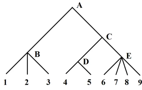
There is a third extension of group lasso which generalises overlapping group lasso and bi-level selection, where it is assumed that the variables have a hierarchical structure represented by a rooted treeT. For an illustration, see Figure2.7. A graph is a tree if it is connected and does not contain cycles. A tree is rooted if one of the vertex is designated as the “root” such that the edges have a natural orientation away from this vertex. InT, a vertex of degree1is referred as a “leaf”, which corresponds to an individual predictor. A vertex of degree at least2is referred as an “internal node”. Each internal node represents a clustering of the variables which are leaf nodes of the sub-tree rooted at that internal node. For instance, the sub-tree rooted at internal nodeBcorresponds to a clustering of variables indexed 1, 2, 3; the sub-tree rooted atC corresponds to a clustering of variables indexed
4−9.
LetV denote the set of vertices inT, which include the root, internal nodes, and leaves. The tree-guided group lasso [Kim and Xing, 2010] generalises group lasso to hierarchical groups where the groups are defined as the leaf nodes of the sub-tree rooted at every vertex
v ∈V. Specifically, letRvdenote a group of variables which are the leaves of the sub-tree rooted atv, the tree-guided group lasso penalty is defined as [Kim and Xing,2010,Jenatton et al.,2012]:
Ω(β) =λX
v∈V
Figure 2.7: A toy example of a rooted tree in which the root is vertexA. There are9leaves which correspond to variables indexed1-9. VerticesB, C, D, E are four internal nodes, each representing a clustering of the variables which are leaf nodes of the sub-tree rooted at that internal node.
where wv is the weight assigned to the vertex v which can be either a fixed or tuning parameter, and λ is a non-negative real valued parameter regularising the overall model sparsity. We illustrate the effect of (2.17) using a toy example where we take a sub-treeT0 ofT rooted at nodeC. By referring to Figure2.7, the vertices setV0ofT0includes internal verticesC,D,E, and the leaf nodes4-9. Therefore:
X v∈V0 wvkβRvk2 =wCkβRCk2+wDkβRDk2+wEkβREk2+ 9 X j=4 wj|βj| (2.18) whereβRC = (β4, β5, ..., β9), βRD = (β4, β5), andβRE = (β6, β7, β8, β9). The first three
terms in the right hand side of (2.18) promote group selection at multiple granularity along the treeT0 and the last summation term of`1norms enables the selection of each individual variable. The weight constant at each node allows us to regularise model sparsity and the grouping structure of the selected variables. The tree structure will guide variable selection such that if the group of variables Rv is regarded unimportant, then all variables which are the leaf nodes of the sub-tree rooted atv attain zero coefficients; on the other hand, if
2.3 Introduction to structured penalties 42
the group of variablesRvis regarded important, then at least one group of variables which branches atvare selected.
2.3.2
Graph-structured penalties
Another way to represent the relationship among the variables is to use a graph G = G(V, E, W), where each vertex in the vertices setV refers to a variable and E is the set of edges which can be either weighted or unweighted. In the case of weighted edges, the weights are represented by the p×p matrixW whose entrieswij are real numbers. The magnitude of the weight quantifies the strength of the pairwise relationship, and the sign describes whether the pair of variables are positively or negatively related. Such a graph structure is often convenient to construct for biological data. For instance, protein-protein interaction networks are available from the Biomolecular Interaction Network Database (BIND) [Alfarano et al., 2005] and many other sources. For another example, gene simi-larity scores can be computed using gene functional annotations from Gene Ontology [ Ash-burner et al.,2000]. A common assumption on the graph is that a pair of variables with large weights are more likely to participate in the same biological process than a pair of variables with small weights, and likewise for variables which are close in the graph comparing with those that are far apart. Hence, encouraging functionally related variables to be selected together seems a promising way to improve model selection accuracy and interpretability.
For convenience, we illustrate the effect of graph-structured penalties in a linear regres-sion model, where the given network is on predictor variables. The estimated coefficients are typically obtained by minimising theβwith respect to the following objective function:
ky−Xβk22+ 2λkβk1 +µN P(β) (2.19) where the lasso penalty induces sparse coefficients and N P(β) is a network-structured penalty which promotes the selection of variables which are close in the network. As in lasso,λregularises model sparsity, while the additional parameterµcontrols the weight of the prior knowledge in coefficient estimation.
The most widely applied choices of N P(β) consist of a Laplacian penalty or some variant of it. We refer to the original Laplacian penalty to that proposed inChung[1997]
which is defined as follows:
N P(β) = X
j>i
|wij|(βi−σ(wij)βj)2 (2.20) whereσ(.)is the sign function defined as in (2.8). Laplacian penalty penalises the weighted squared difference of each pair of predictors. Where the weight|wij|is large, the squared difference is heavily penalised, thus promoting the estimated coefficients to attain similar magnitudes. Before we discuss the generic Laplacian lasso in (2.19), we give some insight of Laplacian penalty here. Firstly, note (2.20) can be neatly written as the product of matrices, namely:
X
j>i
|wij|(βi−σ(wij)βj)2 =βTLβ (2.21) whereLis ap×ppositive definite real valued matrix defined as below:
(L)ij =
(
dj if i=j
−wij if i6=j
(2.22)
anddj is the degree of vertexj:dj =
P
k6=j|wjk|.
Assumingλ = 0in (2.19), the Laplacian estimateβˆLapis obtained by minimising the squared loss plus Laplacian penalty:
ky−Xβk2
2 +µβTLβ (2.23)
whereµis a non-negative regularisation parameter. Since (2.23) is strictly convex, any local minimum is also the global minimum. Therefore a closed form solution can be derived by computing the first derivative of (2.23) and equating it to zero, so that:
ˆ
βLap= (XTX+µL)−1XTy . (2.24)
In general, XTX +µL is invertible even if p > n, hence the closed form solution also holds for high-dimensional data. Note if the networkGdoes not consist of any edge so that
2.3 Introduction to structured penalties 44
Figure 2.8: A simple graphG consisting of3vertices and2edges. The edge weights are both assumed to be1. Using this simple example we show that by encouraging the coef-ficients of neighbouring nodes to have similar magnitude (1-2 and 2-3), Laplacian penalty can also exert the same effect on nodes which are not adjacent (1-3), thus allowing infor-mation to propagate along the whole connected network.
more similar to the identity matrix and(XTX +µI)−1 can be regarded as an extreme de-correlation of the predictors [Hoerl and Kennard, 1970]. Analogously, (XTX +µL)−1 performs a similar de-correlation: asµincreases, the Pearson correlations between predic-tors are less accounted while topological similarities obtain more weights in the estimated coefficients ofβLap.
An interesting feature of Laplacian penalty is that not only it drives predictors which are directly connected in G to have similar coefficients, it can also drive the same effect on variables which are not directly connected. Here we use a toy example to illustrate this feature. We assumep= 3and a networkGas shown in Figure2.8, where bothX1 andX3 are connected toX2but they are not directly connected. For simplicity, we also assume the predictors are independent and the edge weights are both equal to1. As such,Lis defined as: L= 1 −1 0 −1 2 −1 0 −1 1
Letr1, r2, r3 be the correlation coefficient between the three predictors and the responsey, such that(r1, r2, r3)T =XTy. Using (2.24), solution to (2.23) can be written as: