Munich Personal RePEc Archive
Compensations in the Shapley value and
the compensation solutions for graph
games
Béal, Sylvain and Rémila, Eric and Solal, Philippe
24 February 2010
Online at
https://mpra.ub.uni-muenchen.de/20955/
Compensations in the Shapley value and the compensation
solutions for graph games
∗Sylvain Béal†, Eric Rémila‡, Philippe Solal§
February 24, 2010
Abstract
We consider an alternative expression of the Shapley value that reveals a system of compensations: each player receives an equal share of the worth of each coalition he belongs to, and has to compensate an equal share of the worth of any coalition he does not belong to. We give an interpretation in terms of formation of the grand coalition according to an ordering of the players and define the corresponding compensation vector. Then, we generalize this idea to cooperative games with a communication graph. Firstly, we consider cooperative games with a forest (cycle-free graph). We extend the compensation vector by considering all rooted spanning trees of the forest (see Demange [3]) instead of orderings of the players. The associated allocation rule, called the compensation solution, is characterized by component efficiency and relative fairness. The latter axiom takes into account the relative position of a player with respect to his component. Secondly, we consider cooperative games with arbitrary graphs and construct rooted spanning trees by using the classical algorithmsDFSand BFS. If the graph is complete, we show that the compensation solutions associated
with DFS and BFS coincide with the Shapley value and the equal surplus division
respectively.
Keywords: Shapley value, compensations, relative fairness, compensation solution,
DFS,BFS, equal surplus division.
JELClassification number: C72.
1
Introduction
The Shapley value (Shapley [17]) is the most studied allocation rule for cooperative games with transferable utility (TU-games henceforth). One way to interpret the Shapley value consists in considering equally likely orderings of players. For each such ordering, the players enter a bargaining room one by one, and upon entering each player is paid his marginal contribution. This procedure yields the so-called marginal vector, and the Shapley value is the average over all orderings of the players of the marginal vectors.
∗The authors are grateful to Theo Driessen, Amandine Ghintran, Anna Khmelnitskaya and Aymeric
Lardon for stimulating discussions. We have also benefited from comments of seminar participants at Caen University and at the first MINT workshop. Financial support by the Complex Systems Institute of Lyon (IXXI) and the National Agency for Research (ANR) – research program “Models of Influence and Network Theory” ANR.09.BLANC-0321.03 – is gratefully acknowledged.
†Corresponding author. Université de Saint-Etienne, CNRS UMR 5824 GATE Lyon Saint-Etienne,
France. E-mail: [email protected]. Tel: (+33)(0)4.77.42.19.68. Fax: (+33)(0)4.77.42.19.50.
‡Université de Lyon, LIP, UMR 5668 CNRS-ENS Lyon-Université Lyon 1, France. E-mail:
[email protected]. Tél: (+33)(0)4.26.23.38.14. Fax: (+33)(0)4.72.72.80.80
§Université de Saint-Etienne, CNRS UMR 5824 GATE Lyon Saint-Etienne, France. E-mail:
Another less-known interpretation of the Shapley value is due to Eisenman [4]. Eisenman envisages a situation in which the grand coalition is split into a “two-alliances”, i.e two blocks bargaining against each other. This configuration is similar to the original idea with which von Neumann and Morgenstern [14] consider an n-person game as a game between a coalition and its complement. In the two-alliances, each player is paid an equal share of the worth of the coalition he belongs to and must contribute an equal share for the other coalition. The total of these payoffs is then zero. Eisenman considers the step-by-step model in which the first two-alliances is selected at random and then, inductively, one player of the smallest coalition is randomly chosen to grow the largest coalition until the grand coalition is formed. The resulting expected payoff vector is the Shapley value. This approach is close to the interpretation incorporating leaders and followers in each of the two-alliances used by Evans [5] to characterize the Shapley value.1
In this article we introduce another interpretation of the Shapley value, which is similar in spirit to the principle of compensation formulated by Eisenman [4] but preserves Shap-ley’s idea of a one-by-one formation of the grand coalition. More specifically, consider any ordering of the players. The first player enters the room and can claim a payoff equal to the worth he produces, otherwise he can refuse to keep on forming the grand coalition. In order to prevent this failure, the remaining players should pay him this worth, and each of them should be charge an equal share of this compensation. Then, the second player enters the room and forms a coalition with the first player. As before this coalition can ask for a compensation equal to its worth in return for continuing to form the grand coalition. Each of the remaining players should pay an equal share of the compensation and the two entered players should split the compensation into two identical parts. Now repeat these stages until the last player enters the room. At this point the grand coalition eventually forms and each player gets an equal share of its worth. In all but the last stage, the total flow of payoffs is null: the players use a compensation scheme. The whole procedure induces a payoff vector which we call the compensation vector. We show that the Shapley value is the average of the compensation vectors over all orderings of the players.
The second and main part of this article consists in extending the principle of the com-pensation vector from TU-games to cooperative games with a communication graph, the so-called graph games. For the class of graph games, a crucial point is to study how the communication constraints influence the allocation rules. There are at least two ways to measure this impact. In a first approach, the communication constraints determine how a coalition isevaluated. There is no restriction on the formation of coalitions, but if a coalition is not connected through the communication graph, its worth is the sum of the worths of its connected parts. This approach is investigated by Myerson [13] who introduces the Myerson value in order to generalize the Shapley value from TU-games to graph games. The Myerson value is the Shapley value of a graph-restricted TU-game: all orderings of the players are considered, but the worth of unconnected coalitions is evaluated according to their con-nected components. In a second approach, the communication constraints determine how the coalitions are to beformed. Orderings of the players that induce unconnected coalitions are ruled out: the formation of the grand coalition requires a communication at any stage. In order to satisfy the communication constraints, Demange [3] proposes to represent the sequential formation of the grand coalition by a rooted spanning tree of the communication
1Alternative formulations of the Shapley value can be found, among others, in Kleinberg and Weiss [12],
graph. A rooted spanning tree singles out a unique player, called the root, and assigns to each other player a unique superior. Each such rooted spanning tree is a partial order on the player set such that any coalition formed by the arrival of a new player is connected: leaves appear first, then the superiors of the leaves, and so on, up to the root. Demange [3] extends the marginal vector from orderings of the players to rooted spanning trees. This second approach is also studied by Heringset al. [8] who introduce the average tree solution for graph games in which the communication graph is a forest (cycle-free graph). This allo-cation rule is the average of the marginal vectors associated with all rooted spanning trees of the forest. Herings et al. [9] and Baron et al. [1] show how an extension of the average tree solution to arbitrary graph games can be seen as another generalization of the Shapley value.
The principle of the compensation vector can be extended in both ways. The first approach leads immediately to the Myerson value since in the graph-restricted game the average of the compensation vectors associated with all orderings coincides with the Shapley value. In this article we therefore adopt the second approach: the compensation vector is generalized from orderings of the players to rooted spanning trees. We distinguish two cases depending on the presence or absence of cycles in the communication graph.
Firstly, if the communication graph is a forest, each player is the root of exactly one rooted spanning tree. In such a case, we define the compensation solution as the average of the compensation vectors associated with all rooted spanning trees. For this class of graph games, the compensation solution can be characterized by the axioms of component efficiency and relative fairness. The first axiom is standard and requires that the payoffs of the members of a component of any forest add up to the worth of the component. The second axiom originates in the considerable empirical and experimental evidence that the player’s relative payoff position is a significant parameter for evaluating fairness considerations (see for instance Fehr and Schmidt [6] and Ho and Su [10]). This second axiom takes into account this feature: a player not only cares about the payoff allocated to him but also cares about the payoff allocated to relevant reference players. In a forest, it is natural to consider the set of players with whom a player communicates as the set of reference agents. The axiom of relative fairness examines the negotiation for the creation of a link that will merge the two components of the forest of which the two negotiating players are members. The two players drive a look to their component to evaluate their payoff and judge whether they have been treated fairly. We assume that these players use the average payoff in their component as a reference point or benchmark to compare their well-being. Relative fairness says that the relative position of the two players with respect to the average payoff in their pre-existing component should be the same. We show that the compensation solution is the unique allocation rule on the class of forest games that satisfies component efficiency and relative fairness.
that the compensation solution associated with the set of rooted spanning trees created by DFS coincides with the Shapley value when the communication graph is complete. A consequence of this result is that the compensation solution can be seen as a generalization of the Shapley value from TU-games to graph games. We also show that the compensation solution defined with respect to trees created by BFS yields the equal surplus division when the communication graph is complete. These results make a comparison between the Shapley value and the equal surplus division in terms of differences in the formation of the grand coalition. The same question is addressed by van den Brink [18] who provide axiomatizations the equal surplus division that are comparable to the axiomatizations of the Shapley value in the sense that they differ only with respect to a property concerning null players, respectively, nullifying players.
The rest of the article is organized as follows. In section 2, we introduce the compensation vector and prove that the Shapley value is the average over all orderings of the players of the compensation vectors. Section 3 is devoted to the generalization to graph games. Following the usual definitions, we split the results into two subsections. Subsection 3.1 contains the axiomatic characterization for the class of forest games. Subsection 3.2 introduces algorithms
DFS and BFS and proves the connections between the compensation solutions and both the Shapley value and the equal surplus division. Section 4 concludes.
2
Reinterpreting the Shapley value
In order to interpret the formation of the grand coalition as the result of a bargaining process, let us consider any arbitrary 3-player TU-game(N, v)with player setN ={1,2,3}. Assume we have the order(1,2,3): player 1 shows up first, then player 2, and finally player 3 completing the formation of the grand coalition N.
In the first stage, coalition {1} is formed. This coalition can claim a compensation of v({1}) in return for continuing to form N. This claim is a credible threat since {1}
would have to give up the worth v({1}) it produces if the formation of N goes on. In case the remaining players 2 and 3 accept to pay this compensation, then coalition {1} cannot threaten any longer to stop forming N. Both players 2 and 3 should be charged an equal amount v({1})/2 of the compensation.
Next player 2 enters the scene and forms coalition {1,2} with player 1. As before, coalition{1,2}can claim a compensation ofv({1,2})to keep on forming the grand coalition. The remaining player 3 will have to payv({1,2})in order to ensure that N will eventually form, and it seems reasonable to split the obtained compensation v({1,2})equally between players 1 and 2.
Stage 1 Stage 2 Stage 3 Total payoff
Player 1 getsv({1}) gets v({1,2})
2 gets
v({1,2,3})
3 v({1}) +
v({1,2}) 2 +
v({1,2,3}) 3
Player 2 pays v({1})
2 gets
v({1,2}) 2 gets
v({1,2,3})
3 −
v({1}) 2 +
v({1,2}) 2 +
v({1,2,3}) 3
Player 3 pays v({1})
2 pays v({1,2}) gets
v({1,2,3})
3 −
v({1})
2 −v({1,2}) +
v({1,2,3}) 3
Extending this procedure to then-person case, we obtain a compensation vector: at each stage of the formation of N, each of the remaining players pays an equal share of the worth of the currently formed coalition, and the total amount is split equally between the entered players. Moreover, since no ordering is pre-determined for a TU-game, we will average over all possible orderings.
Formal definitions are provided below. Let N = {1, . . . , n} be a finite set of players. A cooperative game with transferable utility on N, or simply TU-game, is a characteristic function v : 2N −→ R such that v(∅) = 0. For each S ∈2N, v(S) is the worth of coalition
S. The set of all TU-games on N is denoted by ΓN. A payoff vector x ∈ Rn on N is an
n-dimensional vector giving a payoff xi ∈Rto each playeri∈N. Anallocation rule onΓN
is a functionf : ΓN −→Rn that assigns a payoff vectorf(v)∈Rn to eachv ∈ΓN. For any
coalition S ∈2N such that|S| ≥2, the notation f
S(v)stands for Pi∈Sfi(v).
An ordering of N is a bijective function π on N, where π(i) is the player at position
i∈ {1, . . . , n}inπ. For any ordering πand any playeri∈N, define the coalition containing player i and the set of its predecessors in π as Sπ
i = {j ∈ N : π−1(j) ≤ π−1(i)}. For any
TU-game v ∈ΓN and any orderingπ, we define thecompensation vector cπ(v)∈Rn as:
∀i∈N, cπi(v) = X
j∈N:i∈Sπ j
v(Sπ j)
|Sπ j|
− X
j∈N:i∈N\Sπ j
v(Sπ j)
n− |Sπ j|
. (1)
For any v ∈ ΓN and any ordering π, the marginal contribution vector mπ(v) ∈ Rn is
defined as mπ
i(v) = v(Siπ)−v(Siπ\{i}) for each i∈ N. The Shapley valueis the allocation
rule Sh that assigns to each TU-game v ∈ ΓN the average of all n! marginal contribution
vectors mπ(v):
∀v ∈ΓN,∀i∈N, Shi(v) =
1 n!
X
π
mπi(v).
Equivalently, the Shapley value is the allocation rule such that:
∀v ∈ΓN,∀i∈N, Shi(v) =
X
S∈2N:i∈S
(n−s)!(s−1)!
n! [v(S)−v(S\{i})], (2)
wheres stands for the cardinality of coalitionS. In a first result, we show that the average, over the set of all possible orderings of N, of the compensation vector cπ(v) is the Shapley
value of the TU-game v ∈ΓN.
Lemma 1 For any v ∈ΓN and any i∈N, it holds that:
Shi(v) =
1 n!
X
π
Proof. For any v ∈ΓN and any i∈N, we have:
1 n!
X
π
cπi(v) =
1 n! X π X
j∈N:i∈Sπ j
v(Sπ j)
|Sπ j|
− X
j∈N:i∈N\Sπ j
v(Sπ j)
n− |Sπ j| = 1 n! X
S∈2N
X
π:∃j∈N,Sπ j=S,i∈S
v(S) s −
X
S∈2N
X
π:∃j∈N,Sπ
j=S,i∈N\S
v(S) n−s
= 1 n! X
S∈2N:i∈S
(n−s)!s!×v(S)
s −
X
S∈2N:i∈N\S
(n−s)!s!× v(S)
n−s
= X
S∈2N:i∈S
(n−s)!(s−1)!
n! ×v(S)−
X
S∈2N:i∈N\S
(n−(s+ 1))!s!
n! ×v(S)
= X
S∈2N:i∈S
(n−s)!(s−1)!
n! [v(S)−v(S\{i})] =Shi(v),
which proves the result.
We conclude this section by the definition of another allocation rule on ΓN that will be
used in section 3.2. It is the equal surplus division ESD, which first assigns to each player
i ∈ N his stand-alone payoff v({i}) and then distributes the remainder of v(N) equally among all players in N:
∀v ∈ΓN,∀i∈N, ESDi(v) = v({i}) +
v(N)−P
j∈Nv({j})
n . (3)
3
Generalization to graph games
Consider a 4-person cooperative game(N, v)withN ={1,2,3,4}and such that the bilateral relationships between the players are represented by an undirected graph(N, L)onN where
L contains the links {1,3}, {2,4} and {3,4}. This graph, drawn on the left side of Figure 1, reflects the communication constraints faced by the players. In order to describe the formation of the grand coalition as the result of a bargaining process similar to the one in section 2, we have to take these constraints into account. In particular, imagine that player 4 is the last player who shows up. If the formation of N is describer by a total order, then coalition {1,2,3} must be formed before the last stage. But {1,2,3} is not a connected coalition. The formation of N with player 4 entering in last position cannot be described by such a total order. However, several partial orders are compatible with the limited communication possibilities. As an example, let us suppose that there are two bargaining rooms simultaneously used for the formation of the grand coalition. In the first room, player 1 shows up first and then player 3. In the second room, player 2 shows up. Finally, player 4 shows up and completes the formation of N by connecting the coalitions {1,3} and {2}
formed in the two rooms. This partial order is represented by a rooted spanning tree of
(N, L) drawn on the right side of Figure 1, where a directed link from i to j means that i
1 3
2 4
1 3
2 4
[image:8.612.80.532.381.512.2](N, L)
Figure 1: A communication graph and a rooted spanning tree
During this process, players and coalitions of players that form can threaten to refuse to continue the formation of the grand coalition. In the first bargaining room coalition {1}
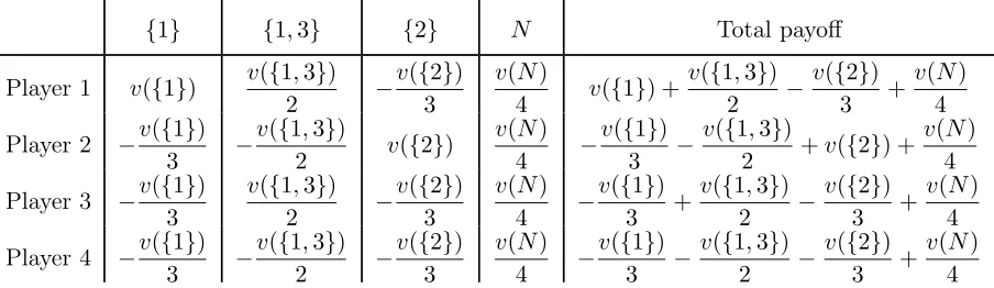
forms in the first step and can credibly claim a worth v({1}). As in the first section, the other players 2, 3 and 4 should bear an equal share of the compensation v({1}) requested by player 1 so as to ensure that the process will go on. Note that the determination of these intermediary payoffs does not rely on whether coalition {2}has already been formed in the second bargaining room since player 2 needs the agreement of player 1 in order to form N. In the second step of the first bargaining room player 3 shows up and forms coalition{1,3}. Players 2 and 4 will have to pay each a compensation v({1,3})/2 to guarantee that this coalition will pursue the formation of the grand coalition, and players 1 and 3 will get each an amount of v({1,3})/2. Continuing in this fashion, we obtain the following payoffs:
{1} {1,3} {2} N Total payoff
Player 1 v({1}) v({1,3})
2 −
v({2}) 3
v(N)
4 v({1}) +
v({1,3}) 2 −
v({2}) 3 +
v(N) 4
Player 2 −v({1})
3 −
v({1,3})
2 v({2})
v(N)
4 −
v({1}) 3 −
v({1,3})
2 +v({2}) +
v(N) 4
Player 3 −v({1})
3
v({1,3})
2 −
v({2}) 3
v(N) 4 −
v({1}) 3 +
v({1,3}) 2 −
v({2}) 3 +
v(N) 4
Player 4 −v({1})
3 −
v({1,3})
2 −
v({2}) 3
v(N) 4 −
v({1}) 3 −
v({1,3}) 2 −
v({2}) 3 +
v(N) 4
This procedure can be extended to anyn-person cooperative game with a communication graph and to any of its rooted spanning trees. We get a payoff vector: at each stage of the (partially ordered) formation of N, each of the players outside of the considered coalition pays an equal share of the worth of this coalition, and the total amount is split equally between the players of the coalition. Moreover, since no particular rooted spanning tree is pre-determined for a TU-game with a communication graph, we will average over the considered set of rooted spanning trees. The resulting allocation rule will be called the compensation solution.
Now let us give formal definitions and notations. An undirected graph is a pair (N, L)
where N is a set of nodes and L is a collection of links, i.e. L ⊆ LN where LN = {{i, j}:
i, j ∈ N, i 6= j}. For ease of notation we write ij instead of {i, j} and L−ij instead of
L\{{i, j}}. For each S ∈ 2N, L(S) = {ij ∈ L : ij ⊆ S} is the set of links between nodes
j are connected in (N, L) if i =j or there exists a path (i1, . . . , ik) with i1 =i and ik =j.
A graph (N, L) is connected if any two nodes are connected. A tree is a connected graph
(N, L) such that for each link ij ∈ L, the graph (N, L−ij) is not connected. A subset S of
N is connected in (N, L) if (S, L(S)) is a connected graph. The empty subset ∅ is trivially connected. A subset C ∈2N is a componentof (N, L)if (C, L(C))is maximally connected,
i.e. if (C, L(C)) is connected and for eachi∈N\C, (C∪ {i}, L(C∪ {i}))is not connected. The collection of components of (N, L), denoted by N/L, forms a partition of N. A graph
(N, L)is a forestif for each component C ∈N/L, (C, L(C))is a tree.
The combination of a TU-game v onN and a communication graph(N, L)is a so-called
graph gameon N, given by a (N, v, L) whereN is the set of players, v is the characteristic function and L the set of links. We fix N and write (v, L) instead of (N, v, L). Let G be any class of graph games on N. An allocation rule onG is a function f that assigns to each
(v, L) ∈ G a payoff vector f(v, L) ∈ Rn. In this article, we consider four classes of graph
games. We denote by GN the class of all graph games on N, by GN∗ the set of all graph
games on N such that (N, L) is a forest, by G∗∗
N be the set of all graph games on N such
that (N, L) is connected and by GLN the class of all graph games on N with a complete
communication graph.
For each component C of a graph(N, L), a spanning treeon C is a minimal set of links that connects all agents in C. A rooted spanning tree onC is a directed graph that arises from this spanning tree by selecting a player r ∈C, called the root, and directing all links away from r. We denote by tr a spanning tree rooted at r ∈ C. For each tr and each
j ∈ C\{r}, there is exactly one directed link (i, j): player i is the unique predecessor of
j and j is a successor of i in tr. Let sri be the possibly empty set of successors of player
i∈C intr. A player j is a subordinate of i intr if there is a directed path from ito j, i.e.
if there is a sequence of distinct players (i1, . . . , ik) such that i1 = i, ik = j, and, for each
q= 1, . . . , k−1,iq+1 ∈sriq. Let S
r
i denote the union of all subordinates of iin tr and {i}.
Now we are ready to adapt the compensation vector for TU-games in the context of graph games. For each graph game(v, L)∈ GN, each componentC ∈N/Land each rooted
spanning tree tr on C, we define the compensation vector as:
∀i∈C, cri(v, L) = X
j∈C:i∈Sr j
v(Sr j)
|Sr j|
− X
j∈C:i∈C\Sr j
v(Sr j)
|C\Sr j|
. (4)
Firstly, the contribution of player i∈C in tr consists in sharing equally the worth v(C)
with the other members of component C. Then, for each coalition Sr
j, j ∈ C\{r}, formed
according to the partial order tr, player i receives a share v(Sjr)/|Sjr| if he belongs to this
coalition or pays v(Sr
j)/|C\Sjr| otherwise. Then we are ready to give the definition of the
compensation solutions.
For the class GN of all graph games onN, we assign to each possible graph a nonempty
set of rooted spanning trees. Define a functionT that assigns to each graph (N, L) and to
each component C ∈ N/L a nonempty set T(L, C) of rooted spanning trees on N. The compensation solution CST(v, L)with respect to T on GN is defined as:
∀(v, L)∈ GN,∀i∈N, CS
T
i (v, L) =
1
|T (L, C)| X
tr∈T(L,C)
For the class of forest games on N, the compensation solution CS on G∗
N is defined as
the average over all rooted spanning trees of the contribution vector (4). Formally:
∀(v, L)∈ GN∗,∀C ∈N/L,∀i∈C CSi(v, L) =
1
|C|
X
r∈C
cri(v, L). (6)
For each graph game (v, L)∈ GN, each component C ∈N/L and each rooted spanning
tree tr on C, Demange [3] defines a marginal vector as follows:
∀i∈C, mr
i(v, L) =v(Sir)−
X
j∈sr i
v(Sr j).
The payoffmr
i(v, L)to playeri∈Cis equal to the worth of the coalition consisting of player
i and all his subordinates in tr minus the sum of the worths of the coalitions consisting of
any successor of player i and all subordinates of this successor intr.
Two other allocation rules for graph games are the average tree solution and the Myerson value. Theaverage tree solutionintroduced by Heringset al. [8] is the allocation rule onG∗
N
that assigns to each forest game the average over all rooted spanning trees of the Demange’s marginal vectors. The Myerson value introduced by Myerson [13] is the allocation rule on
GN that assigns to each graph game (v, L) ∈ GN the Shapley value of the graph-restricted
game vL defined as:
∀S ∈2N, vL(S) = X
T∈S/L(S)
v(T).
To further illustrate the compensation solution, we consider the following example.
Example 1 Consider (v, L) ∈ G∗
N where N = {1,2,3}, L = {12,23} and such that v is
given by:
S {1} {2} {3} {1,2} {1,3} {2,3} {1,2,3}
v(S) 30 0 0 0 0 30 60
Observe that v can be interpreted as the composition of two games: one game on {1}
and one game on {2,3}. The formation of the grand coalition does not create any extra worth compared to the partition {{1},{2,3}}. Therefore, the presence of link 12 in the communication graph does not really matter in terms of worth (the same conclusion would hold if link 13 were to replace 12). All in all, it seems natural that each coalition of the above-mentioned partition gets the worth it produces, i.e. player 1 should obtain 30 and players 2 and 3 should share 30. Moreover, players 2 and 3 are symmetric in v so that they should split equally the payoff 30. The induced vector (30,15,15) is precisely the compensation solution of this graph game, whereas the average tree solution is (30,10,20)
and the Myerson value is (25,10,25).
3.1
The compensation solution for forest games
In this section, we provide a characterization of the compensation solution for forest games. First we need some definitions. For a component C ∈ N/L of a forest (N, L) and a link
ij ∈ L(C), let Ck be the component in (N, L−ij) containing k, where k = i, j. For each
component C, denote by ∆C
Ci and Cj of the subgraph of (C, L(C)) that are obtained after the deletion of the link ij.
In order to characterize the Myerson value, Myerson [13] considers two axioms for the class of all graph games.
Component efficiency. For each(v, L)∈ GN and each C ∈N/L, it holds that
fC(v, L) = v(C).
Fairness. For each (v, L)∈ GN and eachij ∈L, it holds that
fi(v, L)−fi(v, L−ij) = fj(v, L)−fj(v, L−ij).
Fairness says that deleting a link between two players yields for both players the same change in payoff. The Myerson value is the unique allocation rule on GN that satisfies
component efficiency and fairness.
In order to characterize the average tree solution on the class of forest games, Herings
et al. [8] consider the following axiom.
Component fairness. For each (v, L)∈ G∗
N, eachC ∈N/L and each ij ∈ L(C), it holds
that
1
|Ci|
fCi(v, L)−fCi(v, L−ij)
= 1
|Cj|
fCj(v, L)−fCj(v, L−ij)
.
Component fairness says that deleting a link between two players yields for both resulting components the same average change in payoff, where the average is taken over the players in the component. The average tree solution is the unique allocation rule onG∗
N that satisfies
component efficiency and component fairness.
In order to characterize the compensation solution on the class of forest games, we in-troduce the following axiom.
Relative fairness. For each(v, L)∈ G∗
N, each C∈N/L and each ij ∈L(C), it holds that
fi(v, L)−
1
|Ci|
fCi(v, L−ij) =fj(v, L)−
1
|Cj|
fCj(v, L−ij).
Relative fairness has the following interpretation. Players i and j are negotiating the creation of link ij. These players are members of the two components Ci and Cj that are
about to merge. Rather than focusing solely on their allocation changes as in the axiom of fairness, the two playersiandj drive a look to their component to evaluate their payoff and judge whether they have been treated fairly. They care about their relative position with respect to their component. The average payoff in their component is used as a reference point for these players to compare their well-being. Relative fairness says that the relative position of players i and j with respect to average payoff in their pre-existing components
Ci and Cj should be the same. As such, relative fairness shares with the axiom of fairness
the feature that the negotiating players are those involved in the considered link. The axiom of relative fairness also shares with the axiom of component fairness the feature that the payoffs of two involved components are relevant for the creation of a link.
The next two results show that the compensation solution given by (6) is the unique allocation rule on G∗
Theorem 1 On the class G∗
N, there is a unique allocation rule that satisfies component
efficiency and relative fairness.
Proof. Suppose thatf satisfies the two axioms onG∗
N. Pick any(v, L)∈ GN∗, anyC ∈N/L
and any ij ∈ L(C). Note that Ci ∈ N/L−ij and Cj ∈ N/L−ij. Thus component efficiency
of f yields
fCi(v, L−ij) =v(Ci) and fCj(v, L−ij) =v(Cj), (7)
so that relative fairness becomes
fi(v, L)−fj(v, L) =
1
|Ci|
v(Ci)−
1
|Cj|
v(Cj), (8)
with the convention that i < j. Therefore, we obtain |L| equations of the form (8). In addition, we also have |N/L| = |N| − |L| equations given by component efficiency. Let us show that this system of n equations has a unique solution. Consider the matrix A of coefficients given by these n equations. Specifically, for each C ∈ N/L, let aC be the row
of A corresponding to the axiom of component efficiency for component C, i.e. aC
i = 1 for
each i∈C and aC
i = 0 for eachi∈N\C. For each link ij ∈L such that i < j, let a(i,j) be
the row ofAcorresponding to equation (8) associated with linkij,i.e. ai(i,j) = 1,a(ji,j) =−1
and a(ki,j) = 0 for each k ∈N\{i, j}.
We have to prove that the rank of A isn,i.e. that the vector space A generated by the rows of A is Rn. In order to prove this result, we show that, for each i ∈N, the vector bi,
defined by bi
i = 1 and bij = 0 for each j ∈ N\{i} (the ith vector of the canonical basis of Rn) is an element of A.
For each row a(i,j) of A, we first define the n-dimensional vector a(j,i) as: a(j,i)=−a(i,j). Afterwards, we extend the definition of a(i,j) from pairs of linked players to any pair of players in a component as follows. Consider any component C ∈ N/L. Recall that for each C ∈ N/L and each i, j ∈ C, there is a unique path from i to j, which we denote by
(i1, . . . , ik). For eachj ∈C\{i}, create the n-dimensional vector a(i,j) as
a(i,j) =
k−1
X
q=1
a(iq,iq+1).
Thus a(ii,j) = 1, a(ji,j) =−1 and a(ki,j) = 0 for eachk ∈ N\{i, j}. Obviously, the vector a(i,j) is element ofA. Next, for each componentC ∈N/Land eachi∈C, one easily checks that:
bi = 1
|C|
X
j∈C\{i}
a(i,j)+aC
,
which implies that bi is element of A. Thus the rank of A is n, which implies that A is
invertible. Therefore f is uniquely determined.
Theorem 2 On the class G∗
N, the compensation solution given by (6) satisfies component
Proof. Consider any (v, L) ∈ G∗
N and any C ∈ N/L. For a given rooted spanning tree tr
onC, we have:
X
i∈C
cri(v, L) = X
i∈C
X
j∈C:i∈Sr j
v(Sr j)
|Sr j|
− X
j∈C:i∈C\Sr j
v(Sr j)
|C\Sr j|
= X
j∈C
X
i∈Sr j
v(Sr j)
|Sr j|
− X
i∈C\Sr j
v(Sr j)
|C\Sr j|
= v(Srr) + X
j∈C\{r}
|Sjr|v(S
r j)
|Sr j|
− |C\Sjr| v(S
r j)
|C\Sr j|
= v(Sr r)
= v(C).
Therefore,
X
i∈C
CSi(v, L) =
1
|C|
X
i∈C
X
r∈C
cri(v, L) = 1
|C|
X
r∈C
X
i∈C
cri(v, L) = 1
|C|
X
r∈C
v(C) = v(C),
which proves that CS verifies component efficiency. In order to show that CS satisfies relative fairness, we have to prove that CSi(v, L)−CSj(v, L) =CSCi(v, L−ij)/|Ci|−CSCj(v, L−ij)/|Cj|
for each ij ∈L. First recall that for each i∈C,
CSi(v, L) =
1
|C|
X
r∈C
X
j∈C:i∈Sr j
v(Sr j)
|Sr j|
− X
j∈C:i∈C\Sr j
v(Sr j)
|C\Sr j|
.
For a coalitionS ⊂C and a rooted spanning treetr onC, note that there existsj ∈C such
thatSr
j =S if and only if the rootr belongs toC\S. Also, note that for a given component
C ∈ N/L, ∆C
L = {Sir : r, i ∈ C, i 6= r}. We can distinguish coalitions in ∆LC according to
whether they contain player i or not in order to rewrite CSi(v, L) as follows:
CSi(v, L) =
1
|C|
v(C) + X
S∈∆C L:i∈S
X
r∈C\S
v(S)
|S| −
X
S∈∆C L:i∈C\S
X
r∈C\S
v(S)
|C\S|
= 1
|C|
v(C) + X
S∈∆C L:i∈S
|C\S|v(S) |S| −
X
S∈∆C L:i∈S
X
r∈S
v(C\S)
|S|
= 1
|C|
v(C) + X
S∈∆C L:i∈S
|C\S|v(S)
|S| −v(C\S)
= 1
|C|
v(C) + X
S∈∆C L:i∈S
1
|S|
|C\S|v(S)− |S|v(C\S)
.
CSj(v, L)is equal to
1
|C|
X
S∈∆C L:i∈S
1
|S|
|C\S|v(S)− |S|v(C\S)
− X
S∈∆C L:j∈S
1
|S|
|C\S|v(S)− |S|v(C\S)
= 1
|C|
X
S∈∆C
L: i∈S,j∈C\S
1
|S|
|C\S|v(S)− |S|v(C\S)
− X
S∈∆C
L: j∈S,i∈C\S
1
|S|
|C\S|v(S)− |S|v(C\S)
.
Observe that the two components Ci and Cj obtained fromC after deleting link ij ∈L(C)
are the unique elements in ∆C
L that contain player i but not player j and player j but not
player i respectively. As a consequence, the previous expression can be rewritten as:
1
|C|
1
|Ci|
|Cj|v(Ci)− |Ci|v(Cj)
− 1 |Cj|
|Ci|v(Cj)− |Cj|v(Ci)
!
= 1
|C|
1
|Ci|
+ 1
|Cj|
|Cj|v(Ci)− |Ci|v(Cj)
= |Cj|v(Ci)− |Ci|v(Cj)
|Ci||Cj|
= v(Ci)
|Ci|
− v(Cj) |Cj|
= 1
|Ci|
CSCi(v, L−ij)−
1
|Cj|
CSCj(v, L−ij),
where the last equality follows from the fact that the compensation solution satisfies
com-ponent efficiency.
We conclude this section by a comparison between the compensation solution, the My-erson value and the average tree solution.
Example 2 Consider the glove graph game (v, L)∈ G∗
N where |N| ≥ 3,L ={{1i}i∈N\{1}}
and such that player 1 has one left-hand glove while players 2, . . . , n have one right-hand glove each. A (left-right) pair is worth 1d. The corresponding function v is determined by the values: v(S) = 1 if 1 ∈ S and |S| ≥ 2 and v(S) = 0 otherwise. The compensation solution assigns payoffs
CS1(v, L) = 2
n and CSi(v, L) =
n−2
n(n−1), i∈N\{1}.
These payoffs tend to 0 whenntends to infinity. On the one hand, every coalition contained in N\{1} has a null worth, which implies that player 1 never has to pay a compensation during the formation of N. Thus, player 1 always obtains a greater payoff than any other player. On the other hand, if the size of the population increases, then player 1 has to share the worth he produces with more players, which explains why his payoff tends to zero when
In this example, the average tree solution assigns payoffs 1 to player 1 and 0 to each
i ∈N\{1}. In fact, a player i ∈N\{1} is decisive only for the two-person coalition {1, i}. But these coalitions of size two are never formed when the formation of N is described by a rooted spanning tree. Therefore, player 1 is the only decisive player along the formation of N and obtains the whole unit of worth whatever the number of players inN.
Finally, the Myerson value assigns payoffs (n−1)/nto player 1 and1/(n(n−1)) to each
i∈N\{1}. The Myerson value converges to the average tree solution asn tends to infinity. The reason is simple. Suppose that the population N greets an extra player, say player
n+ 1. In the graph-restricted game, coalition{1, n+ 1}is the unique new coalition in which player 1 is not the unique decisive player, whereas 2n−1 coalitions in which 1 is a decisive player are added (all coalitions in N ∪ {n+ 1} containing at least players 1 and n+ 1). In average, player 1 is more decisive after the arrival of the extra player than before.
In this example and in example 1, the compensation solution seems be to a little bit more egalitarian than the Myerson value and the average tree solution. We do not know whether this observation remains valid for a large class of situations.
3.2
The compensation solution for arbitrary graph games
In this section we study the compensation solutions for arbitrary graph games. The defini-tion of the compensadefini-tion soludefini-tions relies on the creadefini-tion of nonempty sets of rooted spanning trees on a communication graph. A general algorithm, called Tree-Growing, is given for constructing spanning trees of a given graph (see Gross and Yellen [7]). It consists in grow-ing a subtree, one link and one player at a time. Then, two particular instances of this algorithm will be considered.
The algorithm introduced in this section can be easily applied to the connected compo-nents of a non-connected graph. Because the compensation vector (4) can be decomposed by the components of a graph, there is no loss of generality to focus on the class G∗∗
N of all
graph games with a connected communication graph. So consider any connected communi-cation graph (N, L). A pair(S, LS)with S ∈2N\{∅}and LS ⊆L(S) is a subtreeof (N, L)
if (S, LS)is a tree on S. Denote byGany such subtree. For any given subtree Gof a graph
(N, L), the links and players of Gare calledtree links andtree players respectively, and the links and players in (N, L) that are not inG are called non-tree linksand non-tree players. A frontier linkforGis a non-tree link with one endpoint in G, called its tree endpoint, and one endpoint not in G, its non-tree endpoint. The graph resulting from adding any frontier link of Gand its associated non-tree endpoint to the subtree G is still a subtree of (N, L).
An essential component of algorithm Tree-Growingis the rule nextLinkwhich selects a frontier link to add to the current subtree. For any subtree G of a graph (N, L), let F
denote the set of frontier links for G. Then the function nextLink((N, L), F) chooses and returns as its value a frontier link in F that is to be added toG. Then, the selected frontier link and its non-tree endpoint are added to the subtreeG. Note that the rulenextLinkmay not be deterministic, depending on how it has been specified to select a frontier link in F. After a frontier link is added to the current subtree, the functionupdateFrontier((N, L), F)
removes from F those links that are no longer frontier links and adds toF those links that have become frontier links. The pseudocode of Tree-Growing is given by Algorithm 1.
Algorithm 1 – Tree-Growing
Input: a finite connected graph (N, L)and a starting player r∈N.
Output: a spanning tree G of (N, L).
Initial conditions: G= ({r},∅), F ={ri∈L:i∈N}. 1: WhileF 6=∅
2: e ←−nextLink((N, L), F)
3: Let i be the non-tree endpoint ofe
4: Add link e and player i to G. 5: updateFrontier((N, L), F)
6: Return treeG.
and Breadth-First Search (BFS). Both algorithms rely on the discovery order. For each subtreeGof(N, L)induced byTree-Growing, thediscovery order is a listing of players in
N in the order in which they are added as subtreeGis grown. Once the spanning treeGhas been returned byTree-Growing, one can easily consider its oriented version tr, where the
root is the starting player r specified as input inTree-Growing. Henceforth, we will refer totr as the output of algorithmTree-Growing. For any output tr of Tree-Growing, the
position of playeriin the discovery order, starting with 0 for playerr, is called thediscovery number of i intr.
In algorithm DFS, nextLink selects a frontier link in F whose tree endpoint has the largest discovery number. In other words, DFS chooses a frontier link incident to the most recently discovered player. If such a link fails to exist, thenDFS“backtracks” to the second most recently discovered player and tries again, and so on. Therefore,DFSdiscovers players “deeper” in the graph whenever possible. In this way,DFScreates spanning trees containing maximal directed paths starting at the rootr. Let DFS(L)denote the nonempty set of all rooted spanning trees of graph (N, L)that DFS creates.
In algorithm BFS, nextLink selects a frontier link in F whose tree endpoint has the smallest discovery number. In other words, algorithm BFS chooses a frontier link incident to the less recently discovered player. If such an link fails to exist, then BFS considers the second less recently discovered player and tries again, and so on. Therefore, BFS explores the graph by selecting frontier links incident to players as close to the root as possible. In this way, BFS creates shortest directed paths from the root to any other player (see Proposition 4.2.4 in Gross and Yellen [7]). Let BFS(L) denote the nonempty set of all rooted spanning trees of graph (N, L)that BFS creates.
We study the compensation solutions with respect to the set of spanning trees created byDFS and BFS respectively. When the communication graph is complete, the resulting CS solutions are shown to coincide with the Shapley value and the equal surplus division onΓN respectively.
Theorem 3 (i) If (N, L) is a tree, then, for each (v, L) ∈ G∗
N, the compensation solution
defined with respect to DFS(L) and given by (5) is the average ofn compensation vectors and coincides with (6).
(ii) If (N, L) is the complete graph (N, LN), then, for (v, LN)∈ G
LN, the compensation solution defined with respect toDFS(LN)and given by (5) is the average ofn!compensation
Proof. (i) The proof is obvious and is omitted.
(ii) Note that DFS(LN) contains only directed lines, since DFS can always grow the current tree by selecting a frontier link incident to the most recently discovered player. There aren!such directed lines, one for each ordering of the players. In order to see this, fix a starting player r. Then, because the graph is complete, the tree can be grown by visiting any of the (n−1) other players. In the next step, there remain (n−2) unvisited players who can be reached from the most recently visited player. The tree can be grown by any of these players. Continuing in this fashion, it follows that for a given starting player, there are(n−1)!different executions ofDFSand each execution constructs a directed line. Since any of the n players can be chosen as starting player, we obtain the n! directed lines. As a consequence, we get:
CSi(v, LN) =
1 n!
X
tr∈DFS(LN)
cri(v, L)
= 1 n!
X
tr∈DFS(LN)
X
j∈N:i∈Sr j
v(Sr j)
|Sr j|
− X
j∈N:i∈N\Sr j
v(Sr j)
|N\Sr j|
.
Because there exists a bijection between the n! directed lines in DFS(LN) and the n!
orderings π ofN, the previous expression is exactly the formula of the Shapley value given
by Lemma 1.
Theorem 4 (i) If (N, L) is a tree, then, for each (v, L) ∈ G∗
N, the compensation solution
defined with respect to BFS(L) and given by (5) is the average of n compensation vectors and coincides with (6).
(ii) If (N, L) is the complete graph (N, LN), then, for (v, LN)∈ G
LN, the compensation solution defined with respect toBFS(LN)and given by (5) is the average ofncompensation
vectors and coincides with the equal surplus division given by (3).
Proof. (i) The proof is obvious and is omitted.
(ii) Note that for each r ∈ N, any player i∈ N\{r} is at distance 1 of r since (N, LN)
is the complete graph. Hence, for any r∈N, the execution ofBFS on (N, LN)starting at
r yields a unique spanning tree tr in which any playeri ∈N\{r} is a successor of the root
r. The setBFS(LN)containsn such rooted spanning trees, one for eachr∈N. Therefore,
for each i∈N, we have
CSBFS
i (v, LN) =
1 n
X
r∈N
cri(v, LN),
where the compensation vector in tr is then given by
crr(v, LN) = v(N) n −
X
j∈N\{r}
v({j}) n−1
and
cr
i(v, LN) =
v(N)
n +v({i})−
X
j∈N\{i,r}
for each i∈N\{r}. Replacing the compensations cr
i(v, LN), r ∈N, by their above
expres-sions, CSBFS
i (v, LN)becomes
1 n
v(N) n −
X
j∈N\{i}
v({j}) n−1 +
X
r∈N\{i}
v(N)
n +v({i})−
X
j∈N\{i,r}
v({j}) n−1
= 1 n
v(N)− X
j∈N\{i}
v({j})
n−1 + (n−1)v({i})−
X
r∈N\{i} X
j∈N\{i,r}
v({j}) n−1
= 1 n
v(N)− X
j∈N\{i}
v({j})
n−1 + (n−1)v({i})−(n−2)
X
j∈N\{i}
v({j}) n−1
= 1 n
v(N) + (n−1)v({i})− X
j∈N\{i}
v({j})
= v({i}) + v(N)−
P
j∈Nv({j})
n = ESDi(v),
which gives the result.
4
Conclusion
In this article we have introduced the compensation solutions for graph games, which rely on an innovative interpretation of the Shapley value for TU games. The compensation solution can be regarded as a generalization of the Shapley value in the sense that it coincides with the Shapley value if the communication graph is complete. For the subclass of forest games we have provided an axiomatic characterization of the compensation solution. One important issue that is not addressed in this article is the stability of the compensation solutions. The compensation solution for forest games belongs to the core of the game in Example 1 (in fact it is the center of gravity of the core in this particular example) but not to the core of the glove game in Example 2. Various extensions of the compensation solutions are also left for future works. For instance linear combinations of the compensation vectors or probability distributions over the set of compensation vectors can be studied in the spirit of what do Béal et al. [2] for the the average tree solutions. Finally, axiomatic characterizations of the compensation vector and economic applications would be of greatest interest.2
References
[1] R. Baron, S. Béal, E. Rémila and P. Solal – “Average Tree Solutions and the Distribution of Harsanyi Dividends”, MPRA Paper No. 17909, 2009.
[2] S. Béal, E. Rémila and P. Solal – “Rooted-tree Solutions for Tree Games”, Euro-pean Journal of Operational Research 203 (2010), pp. 404–408.
2van den Brinket al. [19] and Khmelnitskaya [11] provide such results on the Demange’s marginal vector
[3] G. Demange– “On Group Stability in Hierarchies and Networks”,Journal of Political Economy 112 (2004), pp. 754–778.
[4] R. L. Eisenman – “A Profit-sharing Interpretation of Shapley Value for n-Person Games”, Behavioral Science 12 (1967), pp. 396–398.
[5] R. A. Evans – “Value, Consistency, and Random Coalition Formation”, Games and Economic Behavior 12 (1996), pp. 68–80.
[6] E. FehrandK. M. Schmidt– “A Theory of Fairness, Competition and Cooperation”,
Quarterly Journal of Economics 114 (1999), pp. 817–868.
[7] J. L. Gross and J. Yellen – Graph Theory and its Applications, (second edition) Discrete Mathematics and its Application, Series Editor K.H. Rosen, Chapman & Hall/CRC, 2005.
[8] J.-J. Herings, G. van der Laan and D. Talman– “The Average Tree Solution for Cycle Free Games”, Games and Economic Behavior 62 (2008), pp. 77–92.
[9] J.-J. Herings, G. van der Laan, D. TalmanandZ. Yang– “The Average Tree So-lution for Cooperative Games with Communication Structure”, forthcoming inGames and Economic Behavior.
[10] T.-H. Ho andX. Su– “Peer-Induced Fairness in Games”,American Economic Review
99 (2009), pp. 2022–2049.
[11] A. Khmelnitskaya– “Values for Rooted-tree and Sink-tree Digraph Games and Shar-ing a River”, forthcomShar-ing in Theory and Decision.
[12] N. L. Kleinberg and J. H. Weiss– “The Orthogonal Decomposition of Games and an Averaging Formula for the Shapley Value”,Mathematics of Operations Research 11
(1986), pp. 117–124.
[13] R. B. Myerson – “Graphs and Cooperation in Games”, Mathematics of Operations Research 2 (1977), pp. 225–229.
[14] J. von Neumann and O. Morgenstern – The Theory of Games and Economic Behavior, Princeton University Press, Princeton, 1944.
[15] U. G. Rothblum – “Combinatorial Representations of the Shapley Value Based on Average Relative Payoffs”, The Shapley Value: Essays in Honor of Lloyd S. Shapley (A. Roth eds), Cambridge University Press, Cambridge, UK, 1988, pp. 121–126.
[16] L. M. Ruiz, F. Valenciano and J. M. Zarzuelo – “The Family of Least Square Values for Transferable Utility Games”, Games and Economic Behavior 24 (1998), pp. 109–130.
[18] R. van den Brink– “Null or Nullifying Players: The Difference Between the Shapley Value and Equal Division Solutions”,Journal of Economic Theory136(2007), pp. 767– 775.