Munich Personal RePEc Archive
Regime Specific Predictability in
Predictive Regressions
Gonzalo, Jesus and Pitarakis, Jean-Yves
Universidad Carlos III de Madrid, University of Southampton
December 2010
Online at
https://mpra.ub.uni-muenchen.de/29190/
Regime Specific Predictability in Predictive Regressions
∗Jes´us Gonzalo
Universidad Carlos III de Madrid Department of Economics
Calle Madrid 126
28903 Getafe (Madrid) - Spain
Jean-Yves Pitarakis University of Southampton
Economics Division Southampton SO17 1BJ, U.K
December 30, 2010
Abstract
Predictive regressions are linear specifications linking a noisy variable such as stock returns to past values of a more persistent regressor with the aim of assessing the presence of predictability. Key complications that arise are the potential presence of endogeneity and the poor adequacy of asymp-totic approximations. In this paper we develop tests for uncovering the presence of predictability in such models when the strength or direction of predictability may alternate across different eco-nomically meaningful episodes. An empirical application reconsiders the Dividend Yield based return predictability and documents a strong predictability that is countercyclical, occurring solely during bad economic times.
Keywords: Endogeneity, Persistence, Return Predictability, Threshold Models.
∗Gonzalo wishes to thank the Spanish Ministerio de Ciencia e Innovacion, grant SEJ-2007-63098 and CONSOLIDER 2010 (CSD 2006-00016) and the DGUCM (Community of Madrid) grant EXCELECON S-2007/HUM-044 for partially
supporting this research. Pitarakis wishes to thank the ESRC for partially supporting this research through an individual
research grant RES-000-22-3983. Both authors are grateful to Grant Hillier, Tassos Magdalinos, Peter Phillips and Peter
Robinson for very useful suggestions and helpful discussions. Last but not least we also thank seminar participants at
Queen-Mary, LSE, Southampton, Exeter, Manchester and Nottingham, the ESEM 2009 meetings in Barcelona, the SNDE
2010 meeting in Novara and the 2010 CFE conference in London for useful comments. All errors are our own responsability.
Address for correspondence: Jean-Yves Pitarakis, University of Southampton, School of Social Sciences, Economics Division,
1
Introduction
Predictive regressions with a persistent regressor (e.g. dividend yields, interest rates, realised volatility)
aim to uncover the ability of a slowly moving variable to predict future values of another typically noisier
variable (e.g. stock returns, GDP growth) within a bivariate regression framework. Their pervasive
nature in many areas of Economics and Finance and their importance in the empirical assessment of
theoretical predictions of economic models made this particular modelling environment an important and
active area of theoretical and applied research (see for instance Jansson and Moreira (2006) and references
therein).
A common assumption underlying old and new developments in this area involves working within a
model in which the persistent regressor enters the predictive regression linearly, thus not allowing for
the possibility that the strength and direction of predictability may themselves be a function of some
economic factor or time itself. Given this restriction, existing work has focused on improving the quality
of estimators and inferences in this environment characterised by persistence and endogeneity amongst
other econometric complications. These complications manifest themselves in the form of nonstandard
asymptotics, distributions that are not free of nuisance parameters, poor finite sample approximations
etc. Important recent methodological breakthroughs have been obtained in Jansson and Moreira (2006),
Campbell and Yogo (2006), Valkanov (2003), Lewellen (2004) while recent applications in the area of
financial economics and asset pricing can be found in Cochrane (2008), Lettau and Nieuwerburgh (2008),
Bandi and Perron (2008) amongst others.
The purpose of this paper is to instead develop an econometric toolkit for uncovering the presence of
predictability within regression models with highly persistent regressors when the strength or direction
of predictability, if present, may alternate across different economically meaningful episodes (e.g. periods
of rapid versus slow growth, period of high versus low stock market valuation, periods of high versus
low consumer confidence etc). For this purpose, we propose to expand the traditional linear predictive
regression framework to a more general environment which allows for the possibility that the strength of
predictability may itself be affected by observable economic factors. We have in mind scenarios whereby
the predictability induced by some economic variable kicks in under particular instances such as when
the magnitude of the variable in question (or some other variable) crosses a threshold but is useless in
terms of predictive power otherwise. Alternatively, the predictive impact of a variable may alternate in
sign/strength across different regimes. Ignoring such phenomena by proceeding within a linear framework
as it has been done in the literature may mask the forecasting ability of a particular variable and more
generally mask the presence of interesting and economically meaningful dynamics. We subsequently apply
our methodology to the prediction of stock returns with Dividend Yields. Contrary to what has been
doc-umented in the linear predictability literature our findings strongly point towards the presence of regimes
importantly, our analysis also illustrates the fact that the presence of regimes may make predictability
appear as nonexistent when assessed within a linear model.
The plan of the paper is as follows. Section 2 introduces our model and hypotheses of interest.
Section 3 develops the limiting distribution theory of our test statistics. Section 4 explores the finite
sample properties of the inferences developed in Section 3, Section 5 proposes an application and Section
6 concludes. All proofs are relegated to the appendix. Due to space considerations additional Monte-Carlo
simulations and further details on some of the proofs are provided as a supplementary appendix.
2
The Model and Hypotheses
We will initially be interested in developing the limiting distribution theory for a Wald type test statistic
designed to test the null hypothesis of a linear relationship between yt+1 and xt against the following
threshold alternative
yt+1=
(
α1+β1xt+ut+1 qt≤γ α2+β2xt+ut+1 qt> γ
(1)
where xt is parameterized as the nearly nonstationary process
xt = ρTxt−1+vt, ρT = 1− c
T (2)
with c >0,qt =µq+uqt and ut, uqt and vt are stationary random disturbances. The above
parameter-isation allows xt to display local to unit root behaviour and has become the norm for modelling highly
persistent series for which a pure unit root assumption may not always be sensible. The threshold variable
qt is taken to be a stationary process andγ refers to the unknown threshold parameter. Under α1 =α2
andβ1 =β2our model in (1)-(2) coincides with that in Jansson and Moreira (2006) or Campbell and Yogo
(2006) and is commonly referred to as a predictive regression model while under α1 = α2, β1 =β2 = 0
we have a constant mean specification.
The motivation underlying our specification in (1)-(2) is its ability to capture phenomena such as
regime specific predictability within a simple and intuitive framework. We have in mind scenarios whereby
the slope corresponding to the predictor variable becomes significant solely in one regime. Alternatively,
the strength of predictability may differ depending on the regime determined by the magnitude ofqt. The
predictive instability in stock returns that has been extensively documented in the recent literature and
the vanishing impact of dividend yields from the 90s onwards in particular (see Ang and Bekaert (2007)
and also Table 9 below) may well be the consequence of the presence of regimes for instance. Among
the important advantages of a threshold based parameterisation are the rich set of dynamics it allows
to capture despite its mathematical simplicity, its estimability via a simple least squares based approach
and the observability of the variable triggering regime switches which may help attach a “cause” to the
structure can be viewed as an approximation to a much wider family of nonlinear functional forms. In
this sense, although we do not argue that our chosen threshold specification mimics reality we believe
it offers a realistic approximation to a wide range of more complicated functional forms and regime
specific behaviour in particular. It is also interesting to highlight the consequences that a behaviour such
as (1)-(2) may have if ignored and predictability is assessed within a linear specifications instead, say
yt =βxt−1 +ut. Imposing zero intercepts for simplicity and assuming (1)-(2) holds with some γ0 it is
easy to establish that ˆβ→p β1+ (β2−β1)P(qt> γ0). This raises the possibility that ˆβ may converge to a
quantity that is very close to zero (e.g. when P(qt> γ0)≈β1/(β1−β2)) so that tests conducted within
a linear specification may frequently and wrongly suggest absence of any predictability.
Our choice of modelling xt as a nearly integrated process follows the same motivation as in the
lin-ear predictive regression literature where such a choice for xt has been advocated as an alternative to
proceeding with conventional Gaussian critical values which typically provide poor finite sample
approx-imations to the distribution of t statistics. In the context of a stationary AR(1) for instance, Chan
(1988) demonstrates that for values ofT(1−ρ)≥50 the normal distribution offers a good approximation
while forT(1−ρ)≤50 the limit obtained assuming near integratedness works better when the objective
involves conducting inferences about the slope parameter of the AR(1) (see also Cavanagh, Elliott and
Stock (1995) for similar points in the context of a predictive regression model). Models that combine
per-sistent variables with nonlinear dynamics as (1)-(2) offer an interesting framework for capturing stylised
facts observed in economic data. Within a univariate setting (e.g. threshold unit root models) recent
contributions towards their theoretical properties have been obtained in Caner and Hansen (2001) and
Pitarakis (2008).
In what follows the threshold parameterγ is assumed unknown withγ ∈Γ = [γ1, γ2] andγ1 and γ2
are selected such that P(qt ≤ γ1) = π1 > 0 and P(qt ≤ γ2) = π2 < 1 as in Caner and Hansen (2001).
We also define I1t ≡I(qt ≤γ) and I2t ≡I(qt > γ) but replace the threshold variable with a uniformly
distributed random variable making use of the equality I(qt≤γ) =I(F(qt) ≤F(γ))≡I(Ut≤λ). Here
F(.) is the marginal distribution ofqt and Ut denotes a uniformly distributed random variable on [0,1].
Before proceeding further it is also useful to reformulate (1) in matrix format. Lettingydenote the vector
stacking yt+1 andXi the matrix stacking (Iit xtIit) for i= 1,2 we can write (1) asy=X1θ1+X2θ2+u
or y = Zθ+u with Z = (X1 X2), θ= (θ1, θ2) and θi = (αi, βi)′ i = 1,2. For later use we also define X = X1+X2 as the regressor matrix which stacks the constant and xt. It is now easy to see that for
givenγ orλthe homoskedastic Wald statistic for testing a general restriction onθ, sayRθ= 0 is given by
WT(λ) = ˆθ′R′(R(Z′Z)−1R′)−1Rθ/ˆ σˆ2uwith ˆθ= (Z′Z)−1Z′yand ˆσu2 = (y′y−
P2
i=1y′Xi(Xi′Xi)−1Xi′y)/T is
the residual variance obtained from (1). In practice since the threshold parameter is unidentified under the
null hypothesis inferences are conducted using the SupWald formulation expressed as supλ∈[π1,π2]WT(λ)
with π1 =F(γ1) andπ2=F(γ2).
linearity given byH0A:α1=α2, β1=β2. We write the corresponding restriction matrix asRA= [I −I]
withIdenoting a 2×2 identity matrix and the SupWald statistic supλWTA(λ). At this stage it is important
to note that the null hypothesis given byH0Acorresponds to the linear specificationyt+1 =α+βxt+ut+1
and thus does not test predictability per se since xt may appear as a predictor under both the null and
the alternative hypotheses. Thus we also consider the null given by H0B :α1 =α2, β1 =β2 = 0 with the
corresponding SupWald statistic written as supλWTB(λ) where nowRB = [1 0 −1 0,0 1 0 0,0 0 0 1].
Under this null hypothesis the model is given byyt+1=α+ut+1 and the test is expected to have power
against departures from both linearity and predictability. Finally, our framework will also cover the case
whereby one wishes to test the hypothesisHC
0 :β1 =β2 = 0 without restricting the intercept parameters
so that the null is compatible with both α1 =α2 and α1 6=α2. We will refer to the corresponding Wald
statistic asWTC(λ) with the restriction matrix given byRC = [0 1 0 0,0 0 0 1].
3
Large Sample Inference
Our objective here is to investigate the asymptotic properties of Wald type tests for detecting the presence
of threshold effects in our predictive regression setup. We initially obtain the limiting distribution of
WA
T(λ) under the null hypothesis H0A : α1 = α2, β1 = β2. We subsequently turn to the joint null
hypothesis of linearity and no predictability given byH0B :α1 =α2, β1 =β2= 0 and explore the limiting
behaviour of WTB(λ). This is then followed by the treatment of the null given by H0C :β1 =β2 = 0 via
WTC(λ) and designed to explore potential predictability induced byxregardless of any restrictions on the
intercepts.
Our operating assumptions about the core probabilistic structure of (1)-(2) will closely mimic the
assumptions imposed in the linear predictive regression literature but will occasionally also allow for a
greater degree of generality (e.g. Campbell and Yogo (2006), Jansson and Moreira (2006), Cavanagh,
Elliott and Stock (1995) amongst others). Specifically, the innovations vt will be assumed to follow a
general linear process we write as vt= Ψ(L)et where Ψ(L) =P∞j=0ψjLj,P∞j=0j|ψj|<∞ and Ψ(1)6= 0
while the shocks to yt, denoted ut, will take the form of a martingale difference sequence with respect to
an appropriately defined information set. More formally, lettingwet= (ut, et)′ and Ftwqe ={wes, uqs|s≤t}
the filtration generated by (wet, uqt) we will operate under the following assumptions
Assumptions. A1: E[wet|Ftwqe
−1] = 0, E[wetwe′t|F
e
wq
t−1] =Σe >0, suptEwe4it<∞;A2: the threshold variable qt=µq+uqt has a continuous and strictly increasing distribution F(.) and is such that uqt is a strictly
stationary, ergodic and strong mixing sequence with mixing numbers αm satisfyingP∞m=1α
1
m−
1
r <∞for
some r >2.
One implication of assumption A1 and the properties of Ψ(L) is that a functional central limit theorem
(Bu(r), Bv(r))′ with the long run variance of the bivariate Brownian Motion B(r) being given by Ω =
P∞
k=−∞E[w0w′k] = [(ω2u, ωuv),(ωvu, ωv2)] = Σ + Λ + Λ′. Our notation is such thatΣ = [(e σu2, σue),(σue, σe2)]
and Σ = [(σ2u, σuv),(σuv, σ2v)] with σ2v = σ2e
P∞
j=0ψ2j and σuv = σue since E[utet−j] = 0 ∀j ≥ 1 by
assumption. Given our parameterisation of vt and the m.d.s assumption for ut we have ωuv = σueΨ(1)
and ω2v =σe2Ψ(1)2. For later use we also let λvv =P∞k=1E[vtvt−k] denote the one sided autocovariance
so that ω2v = σv2 + 2λvv ≡ σ2eP∞
j=0ψj2 + 2λvv. At this stage it is useful to note that the martingale
difference assumption in A1 imposes a particular structure on Ω. For instance since serial correlation in
utis ruled out we have ω2u=σu2. It is worth emphasising however that while ruling out serial correlation
in ut our assumptions allow for a sufficiently general covariance structure linking (1)-(2) and a general
dependence structure for the disturbance terms drivingxtand qt. The martingale difference assumption
onutis a standard assumption that has been made throughout all recent research on predictive regression
models (see for instance Jansson and Moreira (2006), Campbell and Yogo (2005) and references therein)
and appears to be an intuitive operating framework given that many applications take yt+1 to be stock
returns. Writing Λ =P∞
k=1E[wtwt′−k] = [(λuu, λuv),(λvu, λvv)] it is also useful to explicitly highlight the
fact that within our probabilitic environment λuu= 0 andλuv = 0 due to the m.d.s property of theu′ts
while λvv and λvu may be nonzero.
Regarding the dynamics of the threshold variableqtand how it interacts with the remaining variables
driving the system, assumption A1 requires qt−j’s to be orthogonal tout forj ≥1. Sinceqtis stationary
this is in a way a standard regression model assumption and is crucial for the development of our
asymptotic theory. We note however that our assumptions allow for a broad level of dependence between
the threshold variableqtand the other variables included in the model (e.g. qtmay be contemporaneously
correlated with both ut and vt). At this stage it is perhaps also useful to reiterate the fact that our
assumption about the correlation of qt with the remaining components of the system are less restrictive
than what is typically found in the literature on marked empirical processes or functional coefficient
models such asyt+1 =f(qt)xt+ut+1 which commonly take qt to be independent of ut and xt.
Since our assumptions also satisfy Caner and Hansen’s (2001) framework, from their Theorem 1 we
can write P[tT r=1]utI1t−1/√T ⇒ Bu(r, λ) as T → ∞ with Bu(r, λ) denoting a two parameter Brownian
Motion with covariance σu2(r1∧r2)(λ1 ∧λ2) for (r1, r2),(λ1, λ2) ∈ [0,1]2 and where a∧b ≡ min{a, b}.
Noting that Bu(r,1) ≡ Bu(r) we will also make use of a particular process known as a Kiefer process
and defined as Gu(r, λ) = Bu(r, λ)−λBu(r,1). A Kiefer process on [0,1]2 is Gaussian with zero mean
and covariance function σ2
u(r1∧r2)(λ1∧λ2−λ1λ2). Finally, we introduce the diffusion process Kc(r) =
Rr
0 e(r−s)cdBv(s) withKc(r) such that dKc(r) =cKc(r) +dBv(r) and Kc(0) = 0. Note that we can also
write Kc(r) =Bv(r) +c
Rr
0 e(r−s)cBv(s)ds. Under our assumptions it follows directly from Lemma 3.1 in
3.1 Testing H0A :α1 =α2, β1 =β2
Having outlined our key operating assumptions we now turn to the limiting behaviour of our test statistics.
We will initially concentrate on the null hypothesis given byH0A:α1=α2, β1=β2 and the behaviour of
supλWTA(λ) which is summarised in the following Proposition.
Proposition 1: Under the null hypothesis H0A:α1 =α2, β1 =β2, assumptions A1-A2 and as T → ∞
the limiting distribution of the SupW ald statistic is given by
sup
λ
WTA(λ) ⇒ sup
λ
1
λ(1−λ)σ2
u
Z 1
0
Kc(r)dGu(r, λ)
′Z 1
0
Kc(r)Kc(r)′
−1
×
Z 1
0
Kc(r)dGu(r, λ)
(3)
where Kc(r) = (1, Kc(r))′, Gu(r, λ) is a a Kiefer process andKc(r) an Ornstein-Uhlenbeck process.
Although the limiting random variable in (3) appears to depend on unknown parameters such as the
correlation betweenBu andBv,σu2and the near integration parameterca closer analysis of the expression
suggests instead that it is equivalent to a random variable given by a quadratic form in normalised
Brownian Bridges, identical to the one that occurs when testing for structural breaks in a purely stationary
framework. We can write it as
sup
λ
BB(λ)′BB(λ)
λ(1−λ) (4)
withBB(λ) denoting a standard bivariate Brownian Bridge (recall that a Brownian Bridge is a zero mean
Gaussian process with covariance λ1∧λ2−λ1λ2). This result follows from the fact that the processes
Kc(r) and Gu(r, λ) appearing in the stochastic integrals in (3) are uncorrelated and thus independent
since Gaussian. Indeed
E[Gu(r1, λ1)Kc(r2)] = E[(Bu(r1, λ1)−λ1Bu(r1,1))(Bv(r2) +
c
Z r2
0
e(r2−s)cB
v(s)ds)]
= E[Bu(r1, λ1)Bv(r2)]−λ1E[Bu(r1,1)Bv(r2)] +
c
Z r2
0
e(r2−s)cE[B
u(r1, λ1)Bv(s)]ds− λ1c
Z r2
0
e(r2−s)cE[B
u(r1,1)Bv(s)]ds
= ωuv(r1∧r2)λ1−λ1ωuv(r1∧r2)
+ cλ1
Z r2
0
e(r2−s)c(r
1∧s)ds−cλ1
Z r2
0
e(r2−s)c(r
1∧s)ds= 0.
Given that Kc(r) is Gaussian and independent of Gu(r, λ) and also E[Gu(r1, λ1)Gu(r2, λ2)] = σu2(r1 ∧
r2)((λ1∧λ2)−λ1λ2 we haveR Kc(r)dGu(r, λ)≡N(0, σ2uλ(1−λ)
R
Kc(r)2) conditionally on a realisation
in Park and Phillips (1988)). Obviously the discussion trivially carries through to Kc and Gu since
E[Kc(r2)Gu(r1, λ1)]′ =E[Gu(r1, λ1) Kc(r2)Gu(r1, λ1)]′= [0 0]′.
The result in Proposition 1 is unusual and interesting for a variety of reasons. It highlights an
environment in which the null distribution of the SupWald statistic no longer depends on any nuisance
parameters as it is typically the case in a purely stationary environment and thus no bootstrapping
schemes are needed for conducting inferences. In fact, the distribution presented in Proposition 1 is
extensively tabulated in Andrews (1993) and Hansen (1997) also provides p-value approximations which
can be used for inference purposes. More recently, Estrella (2003) provides exact p-values for the same
distribution. Finally and perhaps more importantly the limiting distribution does not appear to depend
on c the near integration parameter which is another unusual specificity of our framework.
All these properties are in contrast with what has been documented in the recent literature on testing
for threshold effects in purely stationary contexts. In Hansen (1996) for instance the author investigated
the limiting behaviour of a SupLM type test statistic for detecting the presence of threshold
nonlineari-ties in purely stationary models. There it was established that the key limiting random variables depend
on numerous nuisance parameters involving unknown population moments of variables included in the
fitted model. From Theorem 1 in Hansen (1996) it is straightforward to establish for instance that under
stationarity the limiting distribution of a Wald type test statistic would be given byS∗(λ)′M∗(λ)−1S∗(λ)
withM∗(λ) =M(λ)−M(λ)M(1)−1M(λ), andS∗(λ) =S(λ)−M(λ)M(1)−1S(1). HereM(λ) =E[X′
1X1]
and S(λ) is a zero mean Gaussian process with variance M(λ). Since in this context the limiting
dis-tribution depends on the unknown model specific population moments the practical implementation of
inferences is through a bootstrap style methodology.
One interesting instance worth pointing out however is the fact that this limiting random variable
simplifies to a Brownian Bridge type of limit when the threshold variable is taken as exogenous in
the sense M(λ) = λM(1). Although the comparison with the present context is not obvious since xt
is taken as near integrated and we allow the innovations in qt to be correlated with those of xt the
force behind the analogy comes from the fact that xt and qt have variances with different orders of
magnitude. In a purely stationary setup, taking xt as stationary and the threshold variable as some
uniformly distributed random variable leads to results such as Px2tI(Ut≤λ)/T p
→E[x2tI(Ut≤λ)] and
if xt and Ut are independent we also have E[x2tI(Ut ≤ λ)] = λE[x2t]. It is this last key simplification
which is instrumental in leading to the Brownian Bridge type of limit in Hansen’s (1996) framework. If
now xt is taken as a nearly integrated process and regardless of whether its shocks are correlated with
Ut or not we have Px2tI(Ut ≤λ)/T2 ⇒λRKc2(r) which can informally be viewed as analogous to the previous scenario. Heuristically this result follows by establishing that asymptotically, objects interacting
xt/ √
T and (I1t−λ) such as T1 P(√xt
T)
2(I
1t−λ) or T1 P(√xt
T)(I1t−λ) converge to zero (see also Caner
and Hansen (2001, page 1585) and Pitarakis (2008)). This would be similar to arguing that xt/√T and
in the limit.
3.2 Testing H0B :α1 =α2, β1 =β2 = 0
We next turn to the case where the null hypothesis of interest tests jointly the absence of linearity and
no predictive power i.e. we focus on testing HB
0 :α1 =α2, β1 =β2 = 0 using the supremum ofWTB(λ).
The following Proposition summarises its limiting behaviour.
Proposition 2: Under the null hypothesis H0B : α1 = α2, β1 = β2 = 0, assumptions A1-A2 and as
T → ∞, the limiting distribution of the SupWald statistic is given by
sup
λ
WTB(λ) ⇒
R
K∗
c(r)dBu(r,1)
2
σ2
u
R
K∗
c(r)2
+
sup
λ
1
λ(1−λ)σ2
u
Z
K∗c(r)dGu(r, λ)
′Z
K∗cK∗c(r)′
−1Z
K∗c(r)dGu(r, λ)
′
(5)
where K∗c(r) = (1, K∗
c(r))′,Kc∗(r) =Kc(r)−
R1
0 Kc(r)drand the remaining variables are as in Proposition
1.
Looking at the expression of the limiting random variable in (5) we note that it consists of two components
with the second one being equivalent to the limiting random variable we obtained under Proposition 1.
The first component in the right hand side of (5) is more problematic in the sense that it does not
simplify further due to the fact thatK∗
c(r) andBu(r,1) are correlated sinceωuvmay take nonzero values.
However, if we were to rule out endogeneity by setting ωuv = 0 then it is interesting to note that the
limiting distribution of the SupWald statistic in Proposition 2 takes the following simpler form
sup
λ
WTB(λ) ⇒ W(1)2+ sup
λ
BB(λ)′BB(λ)
λ(1−λ) (6)
whereBB(λ) is a Brownian Bridge andW(1) a standard normally distributed random variable. The first
component in the right hand side of either (5) or (6) can be recognised as the χ2(1) limiting distribution of the Wald statistic for testing H0 :β = 0 in the linear specification
yt+1 = α+βxt+ut+1 (7)
and the presence of this first component makes the test powerful in detecting deviations from the null
(see Rossi (2005) for the illustration of a similar phenomenon in a different context).
Our next concern is to explore ways of making (5) operational since as it stands the first component
of the limiting random variable depends on model specific moments and cannot be universally tabulated.
For this purpose it is useful to notice that the problems arising from the practical implementation of (5)
are partly analogous to the difficulties documented in the single equation cointegration testing literature
in (7) despite the presence of endogeneity (see Phillips and Hansen (1990), Saikkonen (1991, 1992)). As
shown in Elliott (1998) however inferences about β in (7) can no longer be mixed normal when xt is a
near unit root process. It is only very recently that Phillips and Magdalinos (2009) (PM09 thereafter)
reconsidered the issue and resolved the difficulties discussed in Elliott (1998) via the introduction of a
new Instrumental Variable type estimator of β in (7). Their method is referred to as IVX estimation
since the relevant IV is constructed solely via a transformation of the existing regressorxt. It is this same
method that we propose to adapt to our present context.
Before proceeding further it is useful to note thatWB
T (λ) can be expressed as the sum of the following
two components
WTB(λ) ≡ σˆ
2
lin
ˆ
σ2
u
WT(β = 0) +WTA(λ) (8)
where WT(β = 0) is the standard Wald statistic for testing H0 :β = 0 in (7). Specifically,
WT(β= 0) =
1 ˆ
σ2
lin
[Pxt−1yt−Tx¯y¯]2
[Px2
t−1−Tx¯2]
(9)
with ¯x = Pxt−1/T and ˆσ2lin = (y′y−y′X(X′X)−1X′y)/T is the residual variance obtained from the
same linear specification. Although not of direct interest this reformulation of WTB(λ) can simplify the
implementation of the IVX version of the Wald statistic since the setup is now identical to that of PM09
and involves constructing a Wald statistic for testing H0 :β = 0 in (7) i.e we replace WT(β = 0) in (8)
with its IVX based version which is shown to be asymptotically distributed as a χ2(1) random variable and independent of the noncentrality parameter c. Note that although PM09 operated within a model
without an intercept, in a recent paper Kostakis, Magdalinos and Stamatogiannis (2010) (KMS10) have
also established the validity of the theory in models with a fitted constant term.
The IVX methodology starts by choosing an artifical slope coefficient, say
RT = 1− cz
Tδ (10)
for a given constant cz andδ <1 and uses the latter to construct an IV generated as ˜zt=RTz˜t−1+ ∆xt
or under zero initialisation ˜zt = Ptj=1RtT−j∆xj. This IV is then used to obtain an IV estimator of β
in (7) and to construct the corresponding Wald statistic for testing H0 :β = 0. Through this judicious
choice of instrument PM09 show that it is possible to clean out the effects of endogeneity even within the
near unit root case and to subsequently obtain an estimator ofβ which is mixed normal under a suitable
choice of δ (i.e. δ∈(2/3,1)) and setting cz= 1 (see PM09, pp. 7-12).
Following PM09 and KMS10 and letting y∗
t,x∗t and ˜zt∗ denote the demeaned versions of yt,xt and ˜zt
we can write the IV estimator as ˜βivx =Py∗
tz˜t∗−1/
P
x∗
t−1z˜t∗−1. Note that contrary to PM09 and KMS10
we do not need a bias correction term in the numerator of ˜βivx since we operate under the assumption
thatλuv= 0. The corresponding IVX based Wald statistic for testingH0 :β = 0 in (7) is now written as
WTivx(β= 0) = ( ˜β
ivx)2(Px∗
t−1z˜t∗−1)2
˜
σ2
u
P
(˜z∗
t−1)2
with ˜σ2u=P(y∗
t −β˜IV Xx∗t−1)2/T. Note that this latter quantity is also asymptotically equivalent to ˆσ2lin
since the least squares estimator of β remains consistent. Under the null hypothesis H0B we also have that these two residual variances are in turn asymptotically equal to ˆσ2u so that ˆσlin2 /σˆu2 ≈1 in (8).
We can now introduce our modified Wald statistic, say WTB,ivx(λ) for testing HB
0 : α1 = α2, β1 =
β2= 0 in (1) as
WTB,ivx(λ) = WTivx(β = 0) +WTA(λ). (12)
Its limiting behaviour is summarised in the following Proposition.
Proposition 3: Under the null hypothesisH0(B) :α1 =α2, β1 =β2 = 0, assumptions A1-A2,δ∈(2/3,1)
in (10) and as T → ∞, we have
sup
λ
WTB,ivx(λ) ⇒ W(1)2+ sup
λ
BB(λ)′BB(λ)
λ(1−λ) (13)
with BB(λ) denoting a standard Brownian Bridge.
Our result in (13) highlights the usefulness of the IVX based estimation methodology since the
re-sulting limiting distribution of the SupWald statistic is now equivalent to the one obtained under strict
exogeneity (i.e. under ωuv = 0) in (6). The practical implementation of the test is also straightforward,
requiring nothing more than the computation of an IV estimator.
3.3 Some Remarks on Testing Strategies and Further Tests
So far we have developed the distribution theory for two sets of hypotheses that we explicitly did not
attempt to view as connected since both may be of interest and considered individually depending on the
context of the research question. The implementation of hypotheses tests in a sequence is a notoriously
difficult and often controversial endeavor which we do not wish to make a core objective of this paper
especially within the nonstandard probabilistic environment we are operating under. Depending on the
application in hand each of the hypotheses we have considered is useful in its own right. If one is
interested in predictability coming from either x or q for instance then H0B : α1 = α2, β1 = β2 = 0
would be a natural choice. A non rejection of this null would stop the investigation and lead to the
conclusion that the data do not support the presence of any form of predictability with some confidence
level. If one is solely interested in the potential presence of regimes in a general sense then a null such as
H0A:α1=α2, β1=β2 may be the sole focus of an investigation.
Naturally, one could also be tempted to combineH0B and H0A within a sequence and upon rejection of HB
0 and a non rejection of H0A argue in favour of linear predictability while a rejection of H0A would
support the presence of nonlinear predictability in a broad sense. In this latter case the rejection could
specification such as yt+1 =α1I(qt≤γ0) +α2I(qt> γ0) +ut+1 in which predictability is solely driven by
the threshold variable qt is compatible with the rejection of bothH0A and H0B. As in most sequentially
implemented tests however one should also be aware that the overall size of such an approach would be
difficult to control since the two tests will be correlated. Even under independence which would allow a
form of size control the choice of individual significance levels is not obvious and may lead to different
conclusions.
Given the scenarios dicussed above and depending on the application in hand it is now also interesting
to explore the properties of a test that focuses solely on slope parameters with its null given byHC
0 :β1 =
β2= 0. Such a null would be relevant if one were solely interested in the linear or nonlinear predictability
induced by x or if one believed on `a priori grounds that α1 6=α2. As in Caner and Hansen (2001) the
practical difficulty here lies in the fact that H0C is compatible with bothα1 =α2 and α1 6=α2.
We letWTC(λ) = ˆθ′R′
C(RC(Z′Z)−1RC)−1RCθ/ˆ σˆ2u denote the Wald statistic for testingH0C within the
unrestricted specification in (1) and for some given λ ∈ (0,1). When we wish to explicitly impose the
constancy of intercepts in the fitted model used to calculateWTC(λ) we will refer to the same test statistic
asWTC(λ|α1 =α2). The latter is computed from the intercept restricted model which in matrix form can
be written as y =Zφe +u withZe = [1x1 x2], φ= (α β1 β2)′ and where the lower-case vectors xi stack
the elements of xtIit fori = 1,2. More specifically WTC(λ|α1 =α2) = ˆφ′Re′(Re(Ze′Ze)−1Re′)−1Reφ/ˆ σ˜2u with
e
R= [0 1 0,0 0 1] and ˜σ2
u referring to the residual variance from the same intercept restricted specification.
Unless explictly stated however WTC(λ) will be understood to be computed within (1). When α1 6=α2
we also denote by ˆλ=F(ˆγ) the least squares based estimator of the threshold parameter obtained from
the null model yt+1 = α1I1t+α2I2t+ut+1 and λ0 = F(γ0) its true counterpart. Note that since this
threshold parameter estimator is obtained within a purely stationary setting of the null model its
T-consistency follows from Gonzalo and Pitarakis (2002). The following Proposition summarises the large
sample behaviour of WTC(λ) under alternative scenarios.
Proposition 4: (i) Under the null hypothesis H0C :β1 =β2= 0, assumptions A1-A2, and if α1 =α2 in
the DGP, we have as T → ∞,
WTC(λ) ⇒
R
K∗
c(r)dBu(r,1)
2
σ2
u
R
Kc∗(r)2 +χ
2(1) (14)
for any constant λ∈(0,1)and similarly for WTC(λ|α1 =α2). (ii) If α1 6=α2 the limiting result in (14)
continues to hold for WTC(λ0) and WTC(ˆλ) but not for any other λ ∈ (0,1). (iii) Under exogeneity the
limiting random variable in (14) is equivalent to a χ2(2).
The above results highlight a series of important facts. When α1 = α2, the Wald statistics WTC(λ) or
WTC(λ|α1 = α2) evaluated at any λ ∈ (0,1) are seen to converge to a random variable that does not
depend on λ. This is obviously no longer the case when α1 6=α2 and is intuitively due to the fact that
is whyWTC(λ) needs to be evaluated at ˆλorλ0 whenα1 6=α2.
One practical and well known limitation of (14) comes from its first component which depends on
the noncentrality parametercin addition to other endogeneity induced nuisance parameters. As pointed
out in Proposition 4(iii) however imposing exogeneity leads to the interesting and unusual outcome of
a simple nuisance parameter free standard distributional result. Thus if we are willing to entertain an
exogeneity assumption our result in Proposition 4 offers a simple and trivial way of conducting inferences
on the β′s.
Naturally and analogously to the framework of Caner and Hansen (2001) our result in Proposition 4(i)
crucially depends on the knowledge thatα1=α2 while the use ofWTC(λ0) orWTC(ˆλ) presume knowledge
that α1 6= α2 so that λ0 becomes a meaningful quantity. Ifα1 6=α2 with the switch occurring at some
λ0, it is straightforward to show that both WTC(λ|α1 =α2) andWTC(λ) will be diverging to infinity with T. In the former case this will be happening because the test is evaluated at some λ6= λ0 in addition
to the fact that the fitted model ignores the shifting intercepts while in the case of WC
T (λ) this will be
happening solely because λ6=λ0. Naturally, if the ad-hoc choice ofλhappens to fall close toλ0 the use
of WTC(λ) may lead to more moderate distortions when α1 6= α2 while continuing to be correct in the
event that α1 = α2. For purely practical reasons therefore it may be preferable to base inferences on
WC
T (λ) instead of WTC(λ|α1 =α2) even if we believe α1 =α2 to be the more likely scenario.
For the purpose of making our result in Proposition 4(iii) operational even under endogeneity it is
again useful to note thatWTC(λ)≈WT(β = 0, λ) +WT(β1=β2, λ) withWT(β = 0, λ) denoting the Wald
statistic for testing β = 0 inyt+1 =α1I1t(λ) +α2I2t(λ) +βxt+ut+1 for a givenλ∈(0,1) and WT(β1 =
β2, λ) the Wald statistic for testing H0 :β1 = β2 in model (1). More formally, letting Z1 = [I1 I2 x],
ψ1 = (α1 α2 β)′ and R1 = [0 0 1] we have WT(β = 0, λ) = ˆψ1′R′1[R1(Z1′Z1)−1R′1]−1R1ψˆ1/σˆ12 where ˆσ12
is the residual variance from y =Z1ψ1+u, and using our notation surrounding (1), WT(β1 =β2, λ) =
ˆ
θ′R′
2[R2(Z′Z)−1R′2]−1R2θ/ˆ σˆu2 forR2= [0 1 0 −1]. Naturally, if one wishes to maintain the assumption
that α1 = α2 we could also focus on WTC(λ|α1 =α2) ≈WT(β = 0|α1 =α2) +WT(β1 =β2, λ|α1 = α2)
with these two components being evaluated on models with fixed intercepts (i.e. yt+1 =α+βxt+ut+1
for WT(β = 0|α1 = α2) and yt+1 = α+β1xtI1t+β2xtI2t+ut+1 for WT(β1 = β2, λ|α1 = α2)). With
e
Z defined as earlier,WT(β1 =β2, λ|α1 =α2) = ˆφ′R′3[R3(Ze′Ze)−1R′3]−1R3φ/ˆ σ˜u2 for R3 = [0 1 −1] while
WT(β = 0|α1 = α2) is as in (9). Note that the above decompositions are valid asymptotically due to
the omission of scaling factors adjacent to WT(β = 0, λ) that converge to 1 in probability under the null
hypothesis (i.e. ˆσ2 1/σˆu2
p
→1 and ˆσ2
lin/σ˜2u p →1).
Given the above decompositions it is now possible to modifyWTC(λ) (and similarly forWTC(λ|α1 =α2))
WT(β = 0, λ) (orWT(β = 0|α1 =α2) when applicable). Specifically, we let
WTC,ivx(λ) = WTivx(β = 0, λ) +WT(β1 =β2, λ)
WTC,ivx(λ|α1 =α2) = WTivx(β = 0|α1 =α2) +WT(β1=β2, λ|α1 =α2) (15)
where Wivx
T (β = 0|α1 = α2) is as in (11) while WTivx(β = 0, λ) is the IVX based Wald statistic for
testing H0 :β = 0 in y =Z1ψ1+u. More specifically, letting ˜z refer to the IVX vector that stacks the
˜
z′
ts this latter Wald statistic is constructed instrumenting Z1 = (I1 I2 x) with Z1 = (I1 I2 z˜) so that
ψ1,ivx = (Z′1Z1)−1Z′1y and WT(β = 0, λ) is then constructed in a manner identical to equation (25) in
PM09.
The purpose of this IVX based step is to ensure that the new limit corresponding to the first component
in the right hand side of (14) isχ2(1) and thus no longer depending on the noncentrality parametercand other endogeneity induced parameters. Due to its independence from the secondχ2(1) component which arises as the limit of WT(β1 = β2, λ) or WT(β1 = β2, λ|α1 = α2) (see the proof of Proposition 4(iii))
we also have the useful outcome that WTC,ivx(λ) ⇒ χ2(2) for some λ∈(0,1) when α
1 =α2 in addition
to WTC,ivx(ˆλ) ⇒ χ2(2) and WTC,ivx(λ0) ⇒ χ2(2) when α1 6= α2. Our simulation based results presented
below document a remarkably accurate match of the finite sample quantiles of WTC,ivx(λ) andWTC,ivx(ˆλ)
with those of the χ2(2) (see Table 7).
Although the above might suggest a unified way of testing HC
0 : β1 =β2 = 0 regardless of whether
α1 = α2 or α1 6= α2 this is not so due to the treatment of λ in the construction of WTC,ivx(λ). When
α1 = α2 and as in Proposition 4 above the test statistic can be evaluated at any constant λ ∈ (0,1).
This is no longer true however if α1 6=α2 with the switch occurring at λ0. In this latter case we have
WTC,ivx(ˆλ) ⇒ χ2(2) and obviously WTC,ivx(λ0) ⇒ χ2(2). When α1 6= α2 evaluating WTC,ivx(.) at some
λ6=λ0 would lead to wrong inferences and similarly whenα1=α2, evaluating the same test statistic at
ˆ
λ would be misleading since ˆλ is not a well defined quantity when α1 = α2. Indeed under α1 =α2, ˆλ
does not converge in probability to a constant and the consequences of this on the bahaviour of the test
statistic are unclear.
4
Finite Sample Analysis
4.1 Testing H0A :α1 =α2, β1 =β2
Having established the limiting properties of the SupWald statistic for testing HA
0 our next goal is to
illustrate the finite sample adequacy of our asymptotic approximation and empirically illustrate our
theoretical findings. It will also be important to highlight the equivalence of the limiting results obtained
in Proposition 1 to the Brownian Bridge type of limit documented in Andrews (1993) and for which Hansen
evaluate the size properties of our tests as well.
Our data generating process (DGP) underH0A is given by the following set of equations
yt = α+βxt−1+ut xt =
1− c
T
xt−1+vt
vt = ρvt−1+et, (16)
with ut and et both N ID(0,1) while the fitted model is given by (1) with qt assumed to follow the
AR(1) processqt=φqt−1+uqtwithuqt=N ID(0,1). Regarding the covariance structure of the random
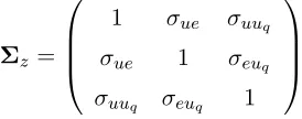
disturbances, letting zt= (ut, et, uqt)′ andΣz =E[ztzt′], we use
Σz =
1 σue σuuq
σue 1 σeuq
σuuq σeuq 1
which allows for a sufficiently general covariance structure while imposing unit variances. Note also that
our chosen covariance matrix parameterisation allows the threshold variable to be contemporaneously
correlated with the shocks to yt. All our H0A based size experiments use N = 5000 replications and set
{α, β, ρ, φ} = {0.01,0.10,0.40,0.50} throughout. Since our initial motivation is to explore the theoret-ically documented robustness of the limiting distribution of SupW aldA to the presence or absence of
endogeneity, we consider the two scenarios given by
DGP1 : {σue, σuuq, σeuq}={−0.5,0.3,0.4}
DGP2 : {σue, σuuq, σeuq}={0.0,0.0,0.0}.
[image:16.612.237.374.254.308.2]The implementation of all our Sup based tests assume 10% trimming at each end of the sample.
Table 1 below presents some key quantiles of theSupW aldAdistribution (see Proposition 1) simulated
using moderately small sample sizes and compares them with their asymptotic counterparts. Results are
displayed solely for the DGP1 covariance structure since the corresponding figures forDGP2 were almost
Table 1: Critical Values of SupW aldA
DGP1, T = 200 DGP1, T = 400 ∞
c= 1 c= 5 c= 10 c= 20 c= 1 c= 5 c= 10 c= 20
2.5% 2.18 2.21 2.21 2.19 2.31 2.24 2.24 2.27 2.41
5.0% 2.53 2.52 2.57 2.50 2.65 2.63 2.62 2.63 2.75
10.0% 3.01 3.07 2.99 2.99 3.13 3.10 3.11 3.12 3.27
90.0% 10.20 10.46 10.48 10.39 10.28 10.23 10.20 10.30 10.46
95.0% 12.07 12.03 12.13 12.19 11.85 12.05 12.11 12.08 12.17
97.5% 13.82 13.76 13.85 13.84 13.74 13.57 13.91 13.64 13.71
Looking across the different values of c as well as the different quantiles we note an excellent adequacy
of the T=200 and T=400 based finite sample distributions to the asymptotic counterpart tabulated in
Andrews (1993) and Estrella (2003). This also confirms our results in Proposition 1 and provides empirical
support for the fact that inferences are robust to the magnitude of c. Note that with T=200 the values
of (1−c/T) corresponding to our choices ofc in Table 1 are 0.995, 0.975, 0.950 and 0.800 respectively.
Thus the quantiles of the simulated distribution appear to be highly robust to a wide range of persistence
characteristics.
Naturally, the fact that our finite sample quantiles match closely their asymptotic counterparts even
under T=200 is not sufficient to claim that the test has good size properties. For this purpose we
have computed the empirical size of the SupW aldA based test making use of the pvsup routine of
Hansen (1997). The latter is designed to provide approximate p-values for test statistics whose limiting
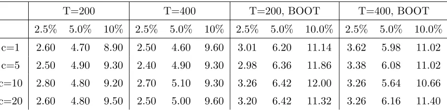
distribution is as in (4). Results are presented in Table 2 below which concentrates solely on the DGP1
[image:17.612.83.535.552.665.2]covariance structure.
Table 2: Size Properties of SupW aldA
T=200 T=400 T=200, BOOT T=400, BOOT
2.5% 5.0% 10% 2.5% 5.0% 10% 2.5% 5.0% 10.0% 2.5% 5.0% 10.0%
c=1 2.60 4.70 8.90 2.50 4.60 9.60 3.01 6.20 11.14 3.62 5.98 11.02
c=5 2.50 4.90 9.30 2.40 4.90 9.30 2.98 6.36 11.86 3.38 6.08 11.02
c=10 2.80 4.80 9.20 2.70 5.10 9.30 3.26 6.42 12.00 3.26 5.64 10.66
c=20 2.60 4.80 9.50 2.50 5.00 9.60 3.20 6.42 11.32 3.26 6.16 11.40
From the figures presented in the two left panels of Table 2 we again note the robustness of the empirical
size estimates ofSupW aldAto the magnitude of the noncentrality parameter. Overall the size estimates
interesting to compare the asymptotic approximation in (4) with that occuring when xt is assumed to
follow an AR(1) with |ρ| < 1 rather than the local to unit root specification we have adopted in this
paper. Naturally, under pure stationarity the results of Hansen (1996, 1999) apply and inferences can
be conducted by simulating critical values from the asymptotic distribution that is the counterpart to
(3) obtained under pure stationarity and following the approach outlined in the aforementioned papers.
This latter approach is similar to an external bootstrap but should not be confused with the idea of
obtaining critical values from a bootstrap distribution. The obvious question we are next interested
in documenting is which approximation works better when xt is a highly persistent process? For this
purpose the two right hand panels of Table 2 above also present the corresponding empirical size estimates
obtained using the asymptotic approximation and its external bootstrap style implementation developed
in Hansen (1996, 1999) and justified by the multiplier central limit theorem (see Van der Vaart and
Wellner (1996)). Although our comparison involves solely the size properties of the test and should
therefore be interpreted cautiously the above figures suggest that the nuisance parameter free Brownian
Bridge based asymptotic approximation does a good job in matching empirical with nominal sizes whenρ
is close to the unit root frontier. Proceeding using Hansen (1996)’s approach on the other hand suggests
a mild oversizeness of the procedure which does not taper off as T is allowed to increase.
Before proceeding further, it is also important to document SupW aldA’s ability to correctly detect
the presence of threshold effects via a finite sample power analysis. Our goal here is not to develop a full
theoretical and empirical power analysis of our test statistics which would bring us well beyond our scope
but to instead give a snapshot of the ability of our test statistics to lead to a correct decision under a
series of fixed departures from the null. All our power based DGPs use the same covariance structure as
our size experiments and are based on the following configurations for {α1, α2, β1, β2, γ} in (1): DGP1A
{−0.03,−0.03,1.26,1.20,0},DGP2A{−0.03,0.15,1.26,1.20,0}andDGP3A{−0.03,0.25,1.26,1.26,0}thus covering both intercept only, slope only and joint intercept and slope shifts. In Table 3 below the figures
represent correct decision frequencies evaluated as the number of times the pvalue of the test statistic
leads to a rejection of the null using a 2.5% nominal level.
Table 3: Power Properties ofSupW aldA
DGP1A DGP2A DGP3A DGP1A DGP2A DGP3A DGP1A DGP2A DGP3A
c= 1 c= 5 c= 10
T = 200 0.73 0.73 0.15 0.39 0.44 0.14 0.20 0.26 0.14
T = 400 0.98 0.98 0.37 0.92 0.93 0.37 0.78 0.82 0.37
T = 1000 1.00 1.00 0.88 1.00 1.00 0.89 1.00 1.00 0.86
We note from Table 3 that power converges towards one under all three parameter configurations
finite sample power even under T = 200 when the slopes are allowed to shift as in DGP1A and DGP2A. It is also interesting to note the negative influence of an increasing c on finite sample power under the
DGPs with shifting slopes. As expected this effect vanishes asymptotically since even for T ≥ 400 the
frequencies across the different magnitudes ofc become very similar.
4.2 Testing H0B :α1 =α2, β1 =β2 = 0
We next turn to the null hypothesis given byH0B:α1=α2, β1=β2 = 0. As documented in Proposition 2
we recall that the limiting distribution of theSupW aldBstatistic is no longer free of nuisance parameters
and does not take a familiar form when we operate under the set of assumptions characterising Proposition
1. However, one instance under which the limiting distribution of theSupW aldB statistic takes a simple
form is when we impose the exogeneity assumption as when considering the covariance structure referred
to asDGP2 above. Under this scenario the relevant limiting distribution is given by (6) and can be easily
tabulated through standard simulation based methods.
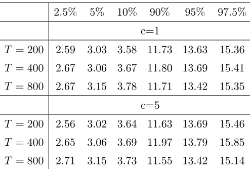
For this purpose, Table 4 below presents some empirical quantiles obtained using T = 200,T = 400
and T = 800 from the null DGP yt= 0.01 +ut. As can be inferred from (6) we note that the quantiles
are unaffected by the chosen magnitude of c and appear sufficiently stable across the different sample
sizes considered. Viewing the T = 800 based results as approximating the asymptotic distribution for
[image:19.612.182.429.451.618.2]instance the quantiles obtained underT = 200 andT = 400 match closely their asymptotic counterparts.
Table 4. Critical Values of SupW aldB under Exogeneity
2.5% 5% 10% 90% 95% 97.5%
c=1
T = 200 2.59 3.03 3.58 11.73 13.63 15.36
T = 400 2.67 3.06 3.67 11.80 13.69 15.41
T = 800 2.67 3.15 3.78 11.71 13.42 15.35
c=5
T = 200 2.56 3.02 3.64 11.63 13.69 15.46
T = 400 2.65 3.06 3.69 11.97 13.79 15.85
T = 800 2.71 3.15 3.73 11.55 13.42 15.14
We next turn to the more general scenario in which one wishes to testHB
0 within a specification that
allows for endogeneity. Taking our null DGP as yt= 0.01 +ut and the covariance structure referred to
asDGP1 it is clear from Proposition 2 that using the critical values from Table 4 will lead to misleading
results. This is indeed confirmed empirically with size estimates forSupW aldBlying about two percentage
points above their nominal counterparts (see Table 5 below). Using our IVX based test statistic in
Results for this experiment are also presented in Table 5 below. Table 5 also aims to highlight the
influence of the choice of the δ parameter in the construction of the IVX variable (see (10)) on the size
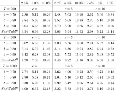
[image:20.612.122.492.163.458.2]properties of the test.
Table 5: Size Properties ofSupW aldB,ivx andSupW aldB under Endogeneity
2.5% 5.0% 10.0% 2.5% 5.0% 10.0% 2.5% 5% 10%
T = 200 c= 1 c= 5 c= 10
δ = 0.70 2.80 5.12 10.26 2.48 5.02 10.40 2.62 5.00 10.34
δ = 0.80 2.84 5.60 10.38 2.52 5.08 10.78 2.70 5.10 10.40
δ = 0.90 3.04 5.48 10.68 2.70 5.20 10.86 2.76 5.32 10.56
SupW aldB 3.54 6.36 12.28 3.06 5.94 11.52 2.98 5.72 11.14
T = 400 c= 1 c= 5 c= 10
δ = 0.70 3.02 5.66 11.06 3.00 5.36 10.60 2.74 5.32 10.14
δ = 0.80 3.14 5.92 11.46 3.14 5.36 10.94 2.82 5.44 10.32
δ = 0.90 3.42 6.28 12.08 3.24 5.52 11.04 2.82 5.48 10.52
SupW aldB 4.28 7.30 13.20 3.46 6.22 11.46 3.08 5.66 11.08
T = 1000 c= 1 c= 5 c= 10
δ = 0.70 2.74 5.14 10.24 2.62 4.96 10.22 2.50 4.72 10.18
δ = 0.80 2.96 5.68 10.74 2.64 5.40 10.12 2.66 4.74 10.62
δ = 0.90 3.30 5.90 11.50 2.92 5.42 10.06 2.64 4.96 10.44
SupW aldB 4.00 6.52 13.18 3.22 5.72 10.74 2.74 5.16 10.74
Overall, we note an excellent match of the empirical sizes with their nominal counterparts. Asδ increases
towards one, it is possible to note a very slight deterioration in the size properties ofSupW aldB,ivx with
empirical sizes mildly exceeding their nominal counterparts. Looking also at the power figures presented
in Table 6 below it is clear that as δ → 1 there is a very mild size power tradeoff that kicks in. This is
perhaps not surprising since as δ → 1 the instrumental variable starts behaving like the original nearly
integrated regressor. Overall, choices of δ in the 0.7-0.8 region appear to lead to very sensible results
within our chosen simulations with almost unnoticeable variations in the corresponding size estimates.
Even under δ= 0.9 and looking across all configurations we can reasonably argue that the resulting size
properties are good to excellent. Finally, the rows labelledSupW aldB clearly highlight the unsuitability
of this uncorrected test statistic whose limiting distribution is as in (5).
Next, we also considered the finite sample power properties of ourSupW aldB,ivx statistic through a
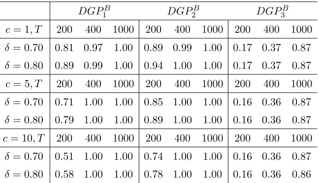
series of fixed departures from the null based on the following configurations for{α1, α2, β1, β2, γ}: DGP1B
Table 6: Power Properties ofSupW aldBivx
DGP1B DGP2B DGP3B c= 1, T 200 400 1000 200 400 1000 200 400 1000
δ= 0.70 0.81 0.97 1.00 0.89 0.99 1.00 0.17 0.37 0.87
δ= 0.80 0.89 0.99 1.00 0.94 1.00 1.00 0.17 0.37 0.87
c= 5, T 200 400 1000 200 400 1000 200 400 1000
δ= 0.70 0.71 1.00 1.00 0.85 1.00 1.00 0.16 0.36 0.87
δ= 0.80 0.79 1.00 1.00 0.89 1.00 1.00 0.16 0.36 0.87
c= 10, T 200 400 1000 200 400 1000 200 400 1000
δ= 0.70 0.51 1.00 1.00 0.74 1.00 1.00 0.16 0.36 0.87
δ= 0.80 0.58 1.00 1.00 0.78 1.00 1.00 0.16 0.36 0.86
The above figures suggest that our modified SupW aldB,ivx statistic has good power properties under
moderately large sample sizes. We again note that violating the null restriction that affects the slopes
leads to substantially better power properties than scenarios where solely the intercepts violate the
equality constraint.
4.3 Testing HC
0 :β1 =β2 = 0
Our initial objective here is to document the accuracy of the χ2(2) approximation for our main IVX
based test statisticWTC,ivx(λ) defined in (15) and designed to make our inferences robust to endogeneity
and to the magnitude of c. When referring to the arguments of our Wald statistics in what follows we
will make use of γ and λ=F(γ) interchangeably. We consider two DGPs having α1 =α2 and α1 6=α2
respectively. In the first case WTC,ivx(γ) is evaluated at an ad-hoc choice of γ while in the second case
we consider WTC,ivx(ˆγ). For ourα1=α2 based experiments we also present the corresponding results for
WTC,ivx(γ|α1 =α2). All our experiments below use δ = 0.7 in the construction of the IVX variable and
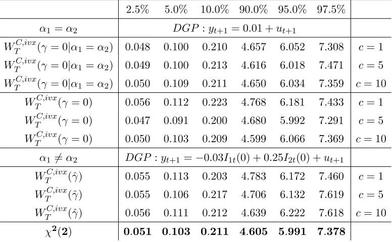
Table 7: Quantiles of WTC,ivx(γ) andWTC,ivx(ˆγ) under Endogeneity (T=400)
2.5% 5.0% 10.0% 90.0% 95.0% 97.5%
α1 =α2 DGP :yt+1 = 0.01 +ut+1
WTC,ivx(γ = 0|α1 =α2) 0.048 0.100 0.210 4.657 6.052 7.308 c= 1
WTC,ivx(γ = 0|α1 =α2) 0.049 0.100 0.213 4.616 6.018 7.471 c= 5
WTC,ivx(γ = 0|α1 =α2) 0.050 0.109 0.211 4.650 6.034 7.359 c= 10
WTC,ivx(γ = 0) 0.056 0.112 0.223 4.768 6.181 7.433 c= 1
WTC,ivx(γ = 0) 0.047 0.091 0.200 4.680 5.992 7.291 c= 5
WTC,ivx(γ = 0) 0.050 0.103 0.209 4.599 6.066 7.369 c= 10
α1 6=α2 DGP :yt+1=−0.03I1t(0) + 0.25I2t(0) +ut+1
WTC,ivx(ˆγ) 0.055 0.113 0.203 4.783 6.172 7.460 c= 1
WTC,ivx(ˆγ) 0.055 0.106 0.217 4.706 6.132 7.619 c= 5
WTC,ivx(ˆγ) 0.056 0.111 0.212 4.639 6.222 7.618 c= 10
χ2(2) 0.051 0.103 0.211 4.605 5.991 7.378
Table 7 above highlights how good a job the IVX based transformation of our original Wald statistic
is doing in matching the theoretical quantiles of the χ2(2) distribution even under a moderately large
sample size such asT = 400. Under the constant intercepts scenario we also note thatWTC,ivx(γ|α1=α2)
leads to quantiles marginally closer to those of the χ2(2) when compared with WTC,ivx(γ). This makes intuitive sense since when α1 = α2, WTC,ivx(γ) implements the test within an unnecessarily overfitted
model.
We next assess the finite sample properties of WTC,ivx(γ) through a series of size based experiments
that distinguish across the two scenarios of interest on the intercepts using the same two DGPs as in
Table 7. Results are presented in Table 8 below. Note that as in Table 7 above all our experiments make
use of a DGP with endogeneity. We make use of WTC,ivx(γ) with an ad-hoc choice ofγ for the DGP with
[image:22.612.132.481.600.692.2]α1 =α2 while we useWTC,ivx(ˆγ) for the DGP withα16=α2.
Table 8: Size Properties ofWTC,ivx(γ) and WTC,ivx(ˆγ) under Endogeneity
α1=α2 α16=α2
WTC,ivx(γ = 1) 2.5% 5.0% 10.0% WTC,ivx(ˆγ) 2.5% 5.0% 10.0%
T = 200 3.10 6.20 10.90 T = 200 2.60 5.10 10.50
T = 400 2.80 5.80 11.00 T = 400 2.90 5.10 10.20
T = 1000 2.50 5.10 10.40 T = 1000 2.80 5.30 10.60
Under α1 = α2 our test statistic is evaluated at the ad-hoc choice of γ = 1 and despite a mild
WTC,ivx(γ = 1) is evaluated on the fully unrestricted model (1) despite our knowledge of the DGP having
α1 = α2 (see our discussion following Proposition 4). Results across alternative magnitudes of γ were
very similar and therefore omitted. Similar properties are also observed when α1 6= α2 with the test
statistic evaluated at ˆγ.
5
Regime Specific Predictability of Returns with Valuation Ratios
One of the most frequently explored specification in the financial economics literature has aimed to uncover
the predictive power of valuation ratios such as Dividend Yields for future stock returns via significance
tests implemented on simple linear regressions linking rt+1 toDYt. The econometric complications that
arise due to the presence of a persistent regressor together with endogeneity issues have generated a vast
methodological literature aiming to improve inferences in such models commonly referred to as predictive
regressions (e.g. Valkanov (2003), Lewellen (2004), Campbell and Yogo (2006), Jansson and Moreira
(2006), Ang and Bekaert (2007) among numerous others).
Given the multitude of studies conducted over a variety of sample periods, methodologies, data
definitions and frequencies it is difficult to extract a clear consensus on predictability. From the recent
analysis of Campbell and Yogo (2006) there appears to be statistical support for some very mild DY based
predictability with the latter having substantially declined in strength post 1995 (see also Lettau and
Van Nieuwerburgh (2008)). Using monthly data over the 1946-2000 period Lewellen (2004) documented
a rather stronger DY based predictability using a different methodology that was mainly concerned with
small sample bias correction. See also Cochrane (2008) for a more general overview of this literature.
Our goal here is to reconsider this potential presence of predictability through our regime based
methodology focusing on the DY predictor. More specifically, using growth in Industrial Production
(IP) as our threshold variable proxying for aggregate macro conditions our aim is to assess whether
the data support the presence of regime dependent predictability induced by good versus bad economic
times. Theoretical arguments justifying the possible existence of episodic instability in predictability
have been alluded to in the theoretical setting of Menzly, Santos and Veronesi (2004) and more recently
Henkel, Martin and Nardari (2009) explored the issue empirically using Bayesian methods within a
Markov-Switching setup. We will show that our approach leads to a novel view and interpretation of the
predictability phenomenon and that its conclusions are robust across alternative sample periods. Moreover
our findings may provide an explanation for the lack of robustness to the sample period documented in
existing linearity based work. An alternative strand of the recent predictive regression literature or
more generally the forecasting literature has also explored the issue of predictive instability through the
allowance of time variation via structural breaks and the use of recursive estimation techniques. A general
message that has come out from this research is the omnipresence of model instability and the important
(2008) amongst others). Our own research is also motivated by similar concerns but focuses on explicitly
identifying predictability episodes induced by a particular variable such as a business cycle proxy.
Our analysis will be based on the same CRSP data set as the one considered in the vast majority
of predictability studies (value weighted returns for NYSE, AMEX and NASDAQ). Throughout all our
specifications the dividend yield is defined as the aggregate dividends paid over the last 12 months divided
by the market capitalisation and is logged throughout (LDY therefater). For robustness considerations
we will distinguish between returns that include dividends and returns that exclude dividends. Finally,
using the 90-day T-Bills all our inferences will also distinguish between raw returns and their excess
counterparts. Following Lewellen (2004) we will restrict our sample to the post-war period. We will
concentrate solely on monthly data since the regime specific nature of our models would make yearly or
even quarterly data based inferences less reliable due to the potentially very small size of the sample. We
will subsequently explore the robustness of our results to alternative sample periods.
Looking first at the stochastic properties of the dividend yield predictor over the 1950M1-2007M12
period it is clear that the series is highly persistent as judged by a first order sample autocorrelation
coefficient of 0.991. A unit root test implemented on the same series unequivocally fails to reject the
unit root null. The IP growth series is stationary as expected displaying some very mild first order
serial correlation and clearly conforming to our assumptions about qt in (1)-(2). Before proceeding with
the detection of regime specific predictability we start by assessing return predictability within a linear
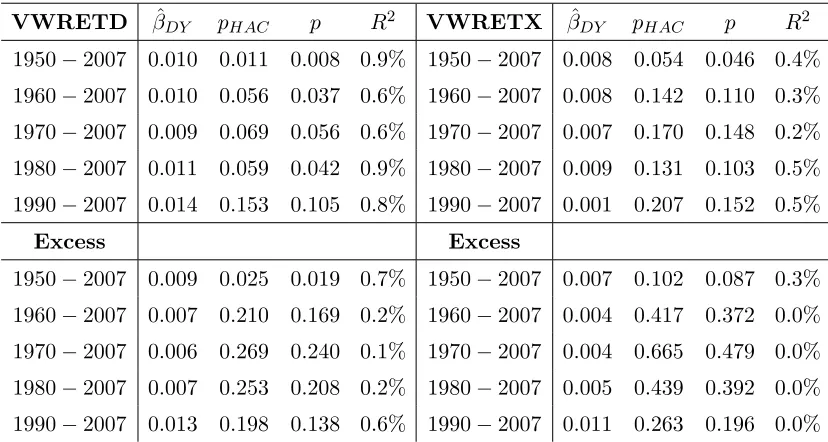
specification as it has been done in the existing literature. Results across both raw and excess returns are
presented in Table 9 below with VWRETD denoting the returns inclusive of dividends and VWRETX
denoting the returns ex-dividends. The columns named as p and pHAC refer to the standard and HAC
[image:24.612.98.512.519.740.2]based pvalues.
Table 9. Linear Predictabilityrt+1 =αDY +βDYLDYt+ut+1
VWRETD βˆDY pHAC p R2 VWRETX βˆDY pHAC p R2
1950−2007 0.010 0.011 0.008 0.9% 1950−2007 0.008 0.054 0.046 0.4%
1960−2007 0.010 0.056 0.037 0.6% 1960−2007 0.008 0.142 0.110 0.3%
1970−2007 0.009 0.069 0.056 0.6% 1970−2007 0.007 0.170 0.148 0.2%
1980−2007 0.011 0.059 0.042 0.9% 1980−2007 0.009 0.131 0.103 0.5%
1990−2007 0.014 0.153 0.105 0.8% 1990−2007 0.001 0.207 0.152 0.5%
Excess Excess
1950−2007 0.009 0.025 0.019 0.7% 1950−2007 0.007 0.102 0.087 0.3%
1960−2007 0.007 0.210 0.169 0.2% 1960−2007 0.004 0.417 0.372 0.0%
1970−2007 0.006 0.269 0.240 0.1% 1970−2007 0.004 0.665 0.479 0.0%
1980−2007 0.007 0.253 0.208 0.2% 1980−2007 0.005 0.439 0.392 0.0%