Optimisation Techniques for Finding Connected
Components in Large Graphs Using GraphX
MAHER TURIFI
University of Salford
School of Computing, Science and Engineering
Submitted in Partial Fulfilment of the Requirements of the Degree of
Doctor of Philosophy
i
Chapter 1:
Contents
LIST OF FIGURES ... IV
LIST OF TABLES ... VII
LIST OF ABBREVIATIONS ...VIII
ABSTRACT ... IX
CHAPTER 1: INTRODUCTION ... 1
1.1 Research Motivation, Aim, and Objectives: ... 3
1.2 Research Methodology: ... 5
1.3 Contributions:... 7
1.4 Outline of the Thesis ... 9
CHAPTER 2: BIG DATA BACKGROUND ... 10
2.1 Big Data: ... 10
2.1.1 Big Data definition ... 10
2.1.2 What is Big Data? ... 11
2.1.3 Components (Three Vs & +V) ... 12
2.1.4 Big Data Benefits ... 14
2.1.5 Associated Challenges with Big Data: ... 14
2.2 Big Data Technologies: ... 15
2.2.1 Hadoop & MapReduce: ... 16
2.2.2 Apache Spark ... 25
CHAPTER 3: LITERATURE REVIEW: ... 30
3.1 Graphs ... 30
3.1.1 Introduction to Network ... 30
3.1.2 Graph Theory: ... 31
3.1.3 Definition ... 32
3.1.4 Characteristics ... 32
3.2 Big Graph ... 34
3.2.1 Big graph History:... 34
3.2.2 Big Graph Systems categorisation ... 37
3.2.3 Big graph system requirements: ... 37
3.2.4 Graph databases ... 39
3.3 Big Graph Processing Systems ... 41
ii
3.4 Approaches in the Developments of Big Graph Processing Systems ... 46
3.5 Summary ... 61
CHAPTER 4: FINDING CONNECTED COMPONENTS IN LARGE GRAPHS ... 62
4.1 What is finding connected components in graphs? ... 62
4.2 Why it is important to study Connected Components algorithms? ... 62
4.3 Application of Connected Components algorithms? ... 63
4.4 Models of study for finding Connected Components: ... 63
4.4.1 In Single machine systems ... 63
4.4.2 In distributed systems ... 64
4.5 Why CC algorithms may perform poorly in practice? ... 66
4.6 Why it is important to use MapReduce in Graph Processing? ... 67
4.7 Previous algorithms for Finding CC in MapReduce ... 68
4.7.1 Using zones to finding connected components ... 68
4.7.2 Pegasus HCC ... 69
4.7.3 Hash-to-Min ... 71
4.7.4 CC-MR ... 73
4.7.5 CCF ... 77
4.7.6 MemoryCC ... 78
4.7.7 CC-MR-mem ... 80
4.7.8 Two-Phase & ALT-OPT ... 84
4.7.9 Cracker ... 86
4.8 Summary ... 87
CHAPTER 5: PROPOSED ALGORITHM ... 90
5.1 Introduction ... 90
5.2 Proposed Improvements ... 91
5.2.1 Graph contraction based on node degree: ... 94
5.2.2 Dynamic evaluation of the degree in the graph: ... 95
5.2.3 Computing local CC in the map phase ... 95
5.3 Preliminaries: ... 97
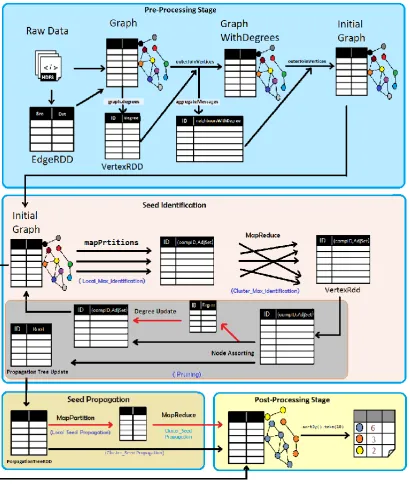
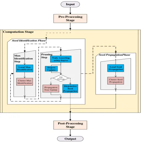
5.4 The Framework Model: ... 97
i. Pre-Processing Stage ... 99
ii. Computing Stage ... 99
5.5 Computing Stage: ... 100
5.5.1 Seed Identification Phase: ... 102
5.5.2 Seed Propagation Phase: ... 116
5.6 Summary ... 118
iii
6.1 Intorduction: ... 119
6.2 Framework Implementation... 121
6.2.1 Pre-Processing Stage ... 122
6.2.2 Computing Stage ... 127
6.2.3 Post-Processing Stage ... 133
CHAPTER 7: EXPERIMENTAL EVALUATION & RESULTS ... 134
7.1 Dataset description ... 134
7.2 Experimental Setup:... 136
7.3 Measuring Metrics: ... 137
7.4 Testing & Results ... 138
7.4.1 Effect of using the Degree Approach to find connected components ... 139
7.4.2 Effect of local Max Identification ... 149
7.4.3 Effect of local Seed Propagation ... 153
7.4.4 Performance of the DS-Pruning ... 154
7.5 Summary ... 156
CHAPTER 8: CONCLUSIONS ... 158
8.1 Introduction: ... 158
8.2 Summary ... 159
8.3 Contributions ... 160
8.4 Limitation ... 162
8.5 Future Works... 163
REFERENCES: ... 165
iv
List of Figures
Figure 1-1: Example of LinkedIn knowledge graph ... 1
Figure 1-2:Overview of the research methodology followed in this thesis ... 6
Figure 2-1: A Mountain of Data represent by multiple of the unit byte[27]. ... 10
Figure 2-2: Big Data Components, the 3 Vs ... 12
Figure 2-3: Hadoop HDFS and MapReduce ... 18
Figure 2-4: Apache Hadoop with YARN. ... 19
Figure 2-5: MapReduce word count Example ... 20
Figure 2-6: Map task and Reduce task in Hadoop... 21
Figure 2-7: MapReduce count word example pseudo code ... 21
Figure 2-8: Apache Spark. ... 25
Figure 2-9: RDD Operations ... 26
Figure 2-10:Spark System[69]... 26
Figure 2-11: RDD dependencies[69]. ... 28
Figure 3-1:GraphX Graph Class ... 58
Figure 3-2: Triplet View ... 58
Figure 3-3: Gelly Graph Class ... 60
Figure 4-1 Hash-to-Min Algorithm[22]. ... 72
Figure 4-2 Reducer of the CC-MR algorithm[13]. ... 75
Figure 4-3 CCF Algorithm[9]... 78
Figure 4-4 MemoryCC Algorithm[119]. ... 80
Figure 4-5 : CC-MR-mem Algorithm (Map Phase) [120]. ... 83
Figure 4-6 Large Start and Small Star operations[14] ... 84
Figure 4-7: The Cracker Algorithm[115] ... 87
v
Figure 5-1: Proposed improvements diagram ... 93
Figure 5-2:Framework Pipeline Model ... 97
Figure 5-3: Algorithm Framework Model ... 98
Figure 5-4: Computation Stage... 101
Figure 5-5: Cracker-Degree Algorithm ... 102
Figure 5-6: Local Max Identification Function ... 106
Figure 5-7: LocalMaxIdentification_Map ... 107
Figure 5-8: ClusterMaxIdentification Function ... 108
Figure 5-9: ClusterMaxIdentification_Map ... 109
Figure 5-10: Node Assorting Flowchart ... 113
Figure 5-11: Node Assorting ... 114
Figure 5-12: Degree Update ... 115
Figure 6-1: adjacencyListGenerator function ... 124
Figure 6-2: findMincCompInSet function ... 124
Figure 6-3: adjacencyListGeneratorDg function ... 126
Figure 6-4: findMaxCompInSet function ... 127
Figure 6-5: Class Diagram ... 128
Figure 6-6: Node Assorting Code ... 130
Figure 7-1: Run-Time for Pregel-Original vs Pregel-Degree ... 140
Figure 7-2: Number of Iterations for Pregel-Original vs Pregel-Degree... 141
Figure 7-3: Iteration vs Reducer Time for Pregel-Original vs Pregel-Degree ... 142
Figure 7-4: Run-Time for Alternating-Original vs Alternating -Degree ... 143
Figure 7-5: Number of Iterations for Alternating-Original vs alternating -Degree ... 143
Figure 7-6: Runtime for the Cracker-Original and Cracker-Degree ... 145
Figure 7-7: Runtime for the Cracker-Original and Cracker-Degree at each step ... 146
vi
Figure 7-9: The number of active nodes at each iteration ... 148
Figure 7-10: Runtime for the Seed Identification Phase ... 150
Figure 7-11: Runtime for for the Seed Identification Phase ... 151
Figure 7-12: Runtime for for the Seed Identification Phase on different datasets ... 152
Figure 7-13: Runtime for the Seed Propagation Phase on different datasets ... 153
vii
List of Tables
Table 4-1: Finding Connected Component Algorithms using MapReduce (n is the number of
nodes, m is the number of edges, d is the diameter) ... 89
Table 7-1: Datasets used in the evaluation ... 135
Table 7-2: Amazon EC2 instances used for the cluster in the evaluation ... 136
Table 7-3: Evaluation Table ... 139
Table 7-4: The number of active nodes at each iteration for synthetic datasets ... 145
Table 7-5: The number of active nodes at each iteration for real-world datasets ... 145
viii
List of abbreviations
BFS Breadth First Search
BSP Bulk Synchronous Parallel
CC Connected Components
DFS Depth First Searches
DHT Distributed Hash-Table
GAS Gather-Sum-Apply-Scatter
HPC High Performance Computers
HDFS Hadoop Distributed File System
MPI Message-Passing Interface
PGM Property Graph Model
PRAM Parallel Random-Access Machine
RDD Resilient Distributed Dataset
RDF Resource Description Framework
ix
Abstract
The problem of finding connected components in undirected graphs has been well studied. It is
an essential pre-processing step to many graph computations, and a fundamental task in graph
analytics applications, such as social network analysis, web graph mining and image
processing. Recently, it has been a major area of interest within the field of large graph
processing. However, much of the research has focused on solving the problem using High
Performance Computers (HPC). In large distributed systems, the MapReduce framework
dominates the processing of big data, and has been used for finding connected components in
big graphs although iterative processing is not directly supported in MapReduce. Current big
data processing systems have developed into supporting iterative processing and providing
additional features other than MapReduce. Moreover, current connected component algorithms
in large distributed processing system only use the traditional approach to choosing the
component identifier based on the lexical ordering of the node ID value. This study investigates
how to enhance the performance of finding connected components algorithm for large graph in
distributed processing system. It uses the approach to considering the graph degree property in
choosing the component identifier, reviewing how this can affect the efficiency of the
algorithm. In the design of our proposed algorithm features provided by current new processing
systems such as moving the computation more toward the data partition in Spark are integrated.
This study thus review how this has affected the performance. The degree approach to choosing
the component identifier is experimentally tested using different algorithms. The study then
applies the proposed approach on the fastest existing algorithm, and experimentally compare
the performance of the connected component algorithm using both the original and our
modified algorithm. The results show that using the degree approach has played a vital role in
the evolution of the graph size during the process, leading to a faster convergence and
significant performance improvement when case vertex pruning is applied in the algorithms.
Furthermore, they demonstrate that in many cases optimising the design of the algorithm with
1
Chapter 1:
Introduction
Big Data was the buzzword of the year 2013[1]. Ever since, the trend towards adopting big
data processing system has increased and it is commonly seen in every aspect of life[2].
Therefore, it has become important for a wide range of scientific and industrial processes,
especially as the cost of storage is decreasing and the ability to capture different kind of data
is growing[3].
In view of the diversity of data acquired nowadays and the massive amount of data stored,
there is a need to find new ways to deal with data beyond the traditional database, such as
handling data that do not usually fit in a single machine memory or disk [4][5]. One approach
is to look at data as a network or a graph with edges connecting things together, those edges
can take different forms of relationships. This metaphor of graph is currently used in many
areas: computer science, economics, sociology, biology, and many more[6]. Almost
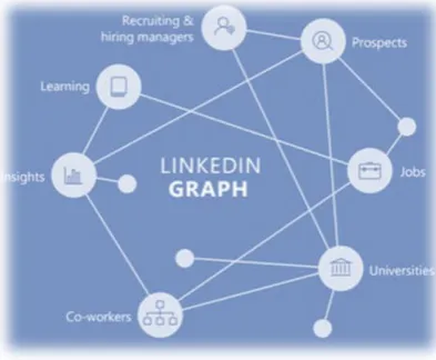
anything can be represented as a graph [7]. Figure 1-1 shows LinkedIn knowledge graph,
where “entities” on LinkedIn, such as members, jobs, titles, skills, companies, geographical
[image:11.595.205.402.535.697.2]locations, schools, etc, and the relationships between them are represented using graph.
Figure 1-1: Example of LinkedIn knowledge graph 1
2
Graphs are considered to be a very flexible data model that can be used to express
relationships between entities, and to recognize local and global characteristics of the
system, and to analyse different features of the complex networks[8] [7] [9].
Extensive research has been carried out on graphs and graph processing, as graphs are one
of the most widely used data representations and have been extensively used to efficiently
process data and extract knowledge[10][7]. However, recent graphs are beyond the ability
of traditional systems to handle, either because the sizes of current graphs are very big, and
they usually do not fit in a machine’s memory, or because current algorithms cannot process
such graphs efficiently, particularly when using the current distributed systems[11].
Our focus in this research is on the problem for finding Connected Components (CC)
efficiently in an undirected graph. A component represents a graph (or subgraph) where any
two vertices inside that graph are connected via paths, and there is no edge that connects any
vertex outside the component[6]. This problem has been well studied, as it is an essential
pre-processing step to many graph computations, and is a building block in complex graph
analysis such as clustering[12][13][14]. It has been a major area of interest within the field
of large graph processing and much of the research so far has focused on solving the problem
using High Performance Computers (HPC), with high computation power and equipped with
very large memory capacity[15].
Large-scale graphs (or big graphs) are usually stored using a distributed file system, like
Hadoop, either in the cloud or locally[16]. Hadoop[17] is an open-source framework that
allows for the distributed storage and processing of large datasets across clusters of
commodity computers. The MapReduce[18][19] framework dominates the processing of
large-scale data on Hadoop, and it is commonly used for mining big graphs[20]. However,
3
works[21][22] show that it is possible to outperform other processing models for finding
connected components using MapReduce. Yet, only a few studies have investigated this
problem in big data distributed system using MapReduce[14].
1.1
Research Motivation, Aim, and Objectives:
Our work builds on the knowledge that current big data processing systems have become
more advanced with features beyond MapReduce. For example, a processing system, like
Spark[23][24], supports iterative processing and provides additional features other than
MapReduce such as data partitioning and caching. Spark also supports graph processing
using GraphX[25], which is an open source Spark API for graph-parallel computation.
Moreover, current connected component algorithms in large distributed processing system
only use the traditional approach in choosing the component identifier for each connected
component based on the lexical ordering of the node ID value. Hence, the aim of this research
is to enhance and optimise the performance of finding connected components in large
undirected graphs using MapReduce.
This could be achieved by addressing the following questions:
Based on the Graph Structure properties, how to increase the efficiency of the algorithm by considering graph structure properties in choosing the component
identifier?
Based on the Processing System properties, how to increase the efficiency of the algorithm in modern processing systems using the new features provided beyond
4
To achieve this research aim, the following objectives have been identified:
1. To adopt a new approach to enhance the performance of CC algorithms by
considering the graph structure in choosing the component identifier. In our case, we
use the degree property in choosing the component identifier for each connected
component.
2. To enhance the performance of the algorithm by using the features provided by the
new current processing systems. In our case, we based our optimisation on the
concept that moving the computation process towards where the data is stored could
help enhance the performance. This is essentially the concept behind MapReduce
also. However, we could benefit further from systems like Spark that provide extra
features by caching the data in memory and controlling the partitioning process
across the cluster.
3. To review current MapReduce algorithms for finding connected components and
choosing the most recent one that outperforms other algorithms to implement
proposed optimisations.
4. To use the best practices and design patterns that have been proven to be efficient in
implementing MapReduce algorithms.
5. To apply the new approach by developing an algorithm for finding connected
components in large-scale graphs and implementing it in the distributed processing
system (GraphX/Spark).
6. To evaluate the efficiency of the new algorithm by analysing its performance using
known tested graph datasets and experimentally compare the performance against
5
1.2
Research Methodology:
Our approach for finding connected components in large scale graphs is based on the degree
of the nodes in the graph and not only the ID of nodes as it is commonly used. Development
and implementation would be applied using GraphX on Spark, an open source Spark API
for graph-parallel computation. The research will apply some of the best practices and design
patterns that have been proven to be efficient in implementing large-scale graph mining
algorithms in MapReduce. Spark’s ability to cache some parts of the data in memory for use
in later iterations will be used. This could help to decrease both the number of iterations and
the intermediate communication load between iterations, and eventually greatly enhance
performance. This could be achieved without losing the ability to expand a graph that does
not fit in memory where Spark can split the cache file on local disks with the need to compute
again.
We adopt an empirical approach method in our research to estimate the effectiveness and
the efficiency of all techniques applied to enhance the performance of finding connected
components algorithm. The approach implemented is tested using large synthetic and
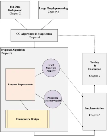
real-world datasets. An overview of our methodology is presented in figure 1-2, with the
corresponding chapter in this thesis.
Initially, we start by exploring Big Data and give overview of the main processing systems
and techniques used with it (Chapter2). In particular, we focus on Apache Hadoop system
and the MapReduce programming model and its limitations, in addition to Apache Spark as
they dominate the big data processing systems currently used. Next, we review graphs and
big graphs, and focus on big graph processing systems (Chapter 3). Our focus in this research
6
using a distributed processing system. Thus, we review available algorithms that use the
MapReduce programming model (Chapter 4).
Proposed Algorithm
Chapter-5
Big Data Background
Chapter-2
Large Graph processing
Chapter-3
CC Algorithms in MapReduce
Chapter-4
Proposed Improvements
Graph Structure Property
Processing System Property
Testing & Evaluation
Chapter-7
Implementation
Chapter-6
[image:16.595.117.494.131.614.2]Framework Design
Figure 1-2:Overview of the research methodology followed in this thesis
Then, we introduce our proposed approach in trying to fulfil the objective of optimising and
enhancing the performance of the connected components algorithm, and approach it from
7
system, such as caching and partitioning in Spark. Afterwards, we design the framework
model for our algorithm (Chapter 5). For implementation, we use the open source system
Spark, namely its graph processing library GraphX, to implements each enhancement
introduced in the designed framework (Chapter 6). Next, we test and evaluate our
implementation using synthetic and real-world datasets and compare the results to the results
of other algorithms. When evaluating the optimisation, we compare our implementation
results with the results of the original unmodified algorithm. For choosing the datasets, we
used open public datasets that often appear in the evaluation of similar algorithms from
related researches. All our tests run in a cloud environment using a virtual cluster (Chapter
7). Finally, we conclude and summarize the result of this study and describe some of the
limitations faced in the process of conducting this research, and then we suggest future work
to overcome some limitations or to further extend this research (Chapter 8).
1.3
Contributions:
The contribution in this thesis are as follows:
(i). Using the node degree approach in finding connected components algorithm:
using the degree approach in choosing the connected component identifier will
always result in less number of iterations until convergence, however it adds some
overload on the system due to the extra work required to calculate the degree for each
node and the increased size of messages due to the attachment of the degree to the
node. Nonetheless, this approach showed significant performance improvement
when applied to algorithms which apply vertex pruning; where unuseful nodes for
the computation are excluded from the process after each iteration. In this kind of
algorithms (Cracker in our case) the number of iterations decreases and the size of
8
(ii). Using the local computation for connected components approach:
Moving more computation towards where the data is stored, and trying to apply
computation on a data partition before the need to do computation on the cluster can
effectively improve the performance of the algorithm. In the case with the Cracker
algorithm, despite the inconsistency in results, in general there is a noticeable
performance improvement especially in the seed propagation phase for the larger datasets. This approach should to be wisely considered and implemented as it could
increase the load on the system and lead to performance degradation.
(iii). Considering different level of computation in the design of the algorithm.
In big data processing system operations are applied at different level, by identifying
the level of processing, and integrating them in the process of the algorithm design
can help to increase the efficiency of the algorithm. For example, start by processing
the data partition, then process the collective data of partitions inside a cluster worker
node, and finally process all the data at the cluster driver node. Customising operation
in the algorithm for each level could increase the performance of the algorithm. In
this study, processing has been customised and applied on the data partitions in the
cluster driver nodes. However, additional operations could be added to process the
data inside a cluster worker node using multi-core structure of the cluster nodes.
(iv). Guidelines to be implemented in different context
It is worth noting that one of the major contribution of this work is to encourage
active researcher in the field to consider features provided by the current new
processing systems in the design of their algorithms using MapReduce. This could
9
1.4
Outline of the Thesis
The content of this thesis is structured as follow: Initially, explore big data processing
systems and techniques (Chapter2). Next, review graphs and big graphs processing systems
(Chapter 3). Review available algorithms for finding connected components using
MapReduce (Chapter 4). Then proposed our approach to enhancing the performance of the
connected components algorithm (Chapter 5). Describe the implementation process for the
proposed enhancement on the fastest existing algorithm (Chapter 6). Next, experimentally
test and evaluate the proposed approach using both the original and modified algorithm
implementation on synthetic and real-world datasets (Chapter 7). Finally, present
10
Chapter 2:
Big Data Background
2.1
Big Data:
2.1.1
Big Data definition
“Big Data” was described as the BUZZWORD for the year 2013-2014 [1], as the discussion
about it is growing with the expectation that the digital universe of data would reach over 35
Zettabytes in 2020 [3][26].
Figure 2-1: A Mountain of Data represent by multiple of the unit byte[27].
In 2015, it was estimated that data reached close to 8 Zettabytes, with a network of 15
billion connected devices. This ocean of data could be imagined as 18 million libraries of
Congress, which are 462 Terabytes each [28]. (See Figure2-1)
For example in the field of social media, the daily generated data in 2011 by Facebook is 10
Terabytes (TB) and by Twitter is 7 TB [3], and in 2012 it was reported that Facebook social
graph contains over a billion nodes and more than 140 billion edges[26]. Multimedia places
a huge load on the internet. Google alone has more than a million servers around the world.
11
In 2016 there were 300 hours of video uploaded to YouTube every minute and more than
1.3 billion unique visitors and over 3.25 billion hours of video watched each month. This is
expected to increase in 2017[30]. In order to exploit the value of this huge amount of data,
organizations must consider three things:
1.Data usually has the characteristics of continuous flow.
2. Analysing the data now is a job that requires significant skill. This is where a Data Scientist is needed, i.e. a professional in analytics and IT who has a deep understanding of the field being investigated and with the management skills and ability to effectively
communicate with decision makers.
3. Real and appropriate outcomes will need both business users and IT people to work
together when analysing large-scale data[31] [32].
2.1.2
What is Big Data?
Big Data is broadly defined as data that is too big, fast, and hard to deal with using
conventional database tools [4][5].
A more technical view is provided by Katal et al.[33], Hunter[34], Kraska[1], Chaudhuri[35]
who define Big Data as data that requires new technologies and architectures. This is
because the database management tools or traditional data processing applications are unable
to process the data in a timely, cost effective way, because it is too large to be stored and
processed and too complex and varied to be analysed and visualised[36]. However,
Venkatram et al. argued that the definition of Big Data varies between organisations and
people based on the data characteristics and the use cases of the data analysis[37]. The name
“Big Data Analytics” is also given to the process of research into Big Data to disclose hidden
12
2.1.3
Components (Three Vs & +V)
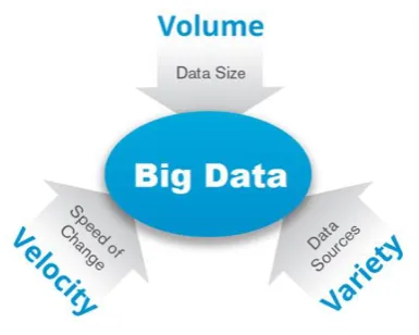
Early in 2001 Doug Laney presented the 3Vs concept in a published research note about the
three challenges of increasing data: data Volume, Variety and Velocity [38].
Later the Three V's became the main components or characteristics that are used to explain
[image:22.595.207.400.231.385.2]what Big data is [33][29][39][40] (figure 2-2).
Figure 2-2: Big Data Components, the 3 Vs2
Volume: is the word associated with “BIG” in big data. It includes the increasing
massive amount of data collected and produced and goes beyond the ability to hold and
process easily.
Variety: data come from many sources. These include, for example, web logs, sensor
data, social media data, emails, images, documents and audio. Data in general comes in
three types: structured, semi-structured and unstructured. Data Variety is probably the
hardest to manage when processing a large amount of data.
Velocity: is concerned with the speed of the data coming from various sources. For
example, streaming data and sensor data or data that is required to be handled in
real-time.
13
In addition to the main 3Vs some researchs [29][33][40] introduced extra Vs, that could
relate to specific business needs and which depend on how the data would be used to
facilitate business decision-making[37]:
Value: how useful is the data in finding useful insights that helps in making better decisions [33] [40] .
Verification: ensuring appropriate data security and that added value should be made to the organization [29] .
Components such as Veracity, Validity and Volatility were also introduced[37].
According to Madden [4] in this explosion of data and the process to adopt the Big Data’s
three Vs, some commercial Relational Databases managed to handle the volume problem
(e.g. Greenplum, Teradata, Vertica). On the other hand, open source systems such as MySQL
and Postgres were unable to manage this problem. However, both commercial and open
source traditional database systems struggle with the velocity and variety problems.
Furthermore, they are not efficient when handling streaming data and lack statistics and
modelling support adoption.
As a result, many research projects attempted to fill the gap between data analysis and data
processing. They usually adopted three approaches:
1. Extending the relational model – for example projects by Oracle and Greenplum.
2. Extending the MapReduce/Hadoop model for example projects like: Apache
Mahout, Spark, HaLoop, Twister, and Daytona.
14
2.1.4
Big Data Benefits
A huge amount of data will be provided to be investigated and analysed by applying big data
analytics in different fields and many sectors. Therefore, rapid advances and discoveries in
many disciplines are expected, in addition to the success and increasing profits for many
enterprises [39]. Big data Analytics can be financially beneficial as well as helping an
organization to have deeper insights into its data whilst enabling faster decision by
processing the data in real time and moving the data processing to where it is stored. When
data scientists and IT experts work closely with business users more efficient solutions to
the problems being studied become possible[28] and this helps decision makers to make
better-informed decisions and develop better strategies[41].
Sagiroglu & Sinanc[29] listed some business benefits that arise when applying big data
analytics. These include more focused marketing, more direct business insights, client based
segmentation, discovery of market opportunities, and automated decision making.
2.1.5
Associated Challenges with Big Data:
Big Data promises beneficial opportunities. However, to be achieved many challenges must
to be addressed. Kraska [1] divided big data issues into:
1. Big Throughput, which concerns the problem associated with storing and manipulating a large amount of data.
2. Big data analytics- which are those issues related to transforming data into knowledge.
Bhatia & Vaswani [39] highlighted the following issues that appear during each phase of big
data analytics: issues of scale, heterogeneity, lack of structure, error-handling, privacy, and
15
For a successful Big Data project, questions about data integration, volume, skill availability
and solution costs should be considered [42]. Katal et al. [33] brought into light various
challenges and issues associated with adopting Big Data solutions. These are:
(a) Technical challenges, which include issues like, fault tolerance, scalability, quality
of data and heterogeneous data.
(b) Storage and processing issues.
(c) Analytical challenges.
(d) Skill requirements.
(e) Privacy, security, data access and sharing of information.
Issues related to privacy, security, data access and sharing of information are very sensitive
issues that all need to be well addressed [33][34] as Big Data Applications could be used for
malevolent intent and will not be in an organization’s best interest. For example, by
aggregating enough information about individuals from their environment with other
information from different sources such as social media, an intrusive profile that has
considerable personal information about an individual could be built [43].
2.2
Big Data Technologies:
Many projects have attempted to develop a distributed system that can handle large-scale
data. For example:
Hadoop [17], is a project to develop open-source software for reliable, scalable and
distributed computing.
Naiad [44], is Microsoft system for data-parallel dataflow computation that focusses
16
Apache Spark[23], [24], is an open source cluster computing system that has
in-memory nature and aims to make data analytics fast.
HPCC (High Performance Computing Cluster)[45], is an open source massively
parallel-processing computing platform that solves Big Data problems.
Pregel [46], is a framework for processing large graphs in which nodes exchange
messages between each other and update their own states in memory. It has an
efficient, scalable and fault-tolerant implementation on clusters of thousands of
commodity computers.
Storm [47], is a free open source distributed real-time computation system. Storm
makes it easy to reliably process unbounded streams of data and can be used with any
programming language.
S4 [48], is a distributed, scalable and fault-tolerant system for processing continuous
unbounded streams of data.
There are other approaches available, which differ according to the problem area or the
application they were designed to address. However,Hadoop is the most dominant platform for distributed processing and many other projects were built using of Hadoop's framework.
Projects can also work side by side with it or use the Hadoop Distributed File System
(HDFS).
2.2.1
Hadoop & MapReduce:
Therefore, this study will describe Hadoop and explain in more detail its programming
model MapReduce with an example. It will then discuss some MapReduce limitations and
detail some of the alternatives available.
Dealing with massive amounts of data is a reality. New software has developed, starting with
17
subsequently proposed by Google [18][19] as a programming model to deal with large
datasets in scalable and distributed fashion [50].
Hadoop is an open-source framework that allows for the distributed processing of large data
sets across clusters of computers using simple programming models. It is based on
MapReduce. HDFS was developed for reliable, scalable, distributed computing [17]. It
allows working with thousands of computers and dealing with petabytes of data [16].
HDFS (Hadoop Distributed File System) is based on the Google File System [49]. It
operates on commodity computers to store data across hundreds of computers. Data nodes
will host files, files are divided into chunks (usually 64 megabytes size), which are replicated
on different disks (usually three times, one disk should be on a different rack). A Master node has a directory that records where each file is stored and replicated [51].
MapReduce gives the programmer the advantages of not needing to consider the details of
data distribution, parallel executing, replication and load balancing. Its programming
concept is familiar [52] and allows parallelised and distributed execution for jobs across
clusters of computers. It requires two functions [51].:
1. Map function, which is defined by the programmer to process Key-Value data. each chunk or more of a given data will be processed by the map function and gives output
as key-value pairs. During the shuffling phase, pairs are collected by a master
controller and sorted by their keys value. They are then divided among reducers in
such a way that each group with the same key goes to the same reducer.
2. Reducer function, takes the key-value pairs and combines all the values associated with the same key and carries out any computation defined by the programmer. It
then outputs the new value. The reducer output could be in key-value pairs to feed
18
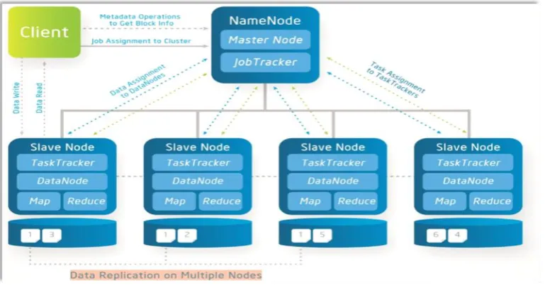
The Hadoop cluster is at least one machine running the Hadoop software. In each cluster,
there is a single master node with a varying number of slave nodes. Slave nodes can act as
both the computing nodes for the MapReduce and as data nodes for the HDFS. This is
[image:28.595.115.500.191.392.2]illustrated in figure 2-3.
Figure 2-3: Hadoop HDFS and MapReduce3
A client submits a job to the master node, which manages it with the slaves in the cluster.
JobTracker controls the MapReduce job, reporting to TaskTracker. TaskTracker will process
the map or reduce operations task. Once the map function has finished a task, the output is
sorted and divided into several groups, which are distributed to the reduce functions.
Reducers may be located on the same node as the mappers or on another node. TaskTracker
reports to JobTracker when it finishes a task. JobTracker then schedules a new task for
TaskTracker [28] [53].
Apache Hadoop is in continuous development and is used in both commercial and research
sectors[53]. Many packages have been developed to run on Apache Hadoop. These include:
Ambri, Avrp, Cassandra, chukwa, Hbase, Hive, Pig, Spark, Tez, ZooKeeper and others.
19
Hbase is a column oriented, scalable, distributed database. Pig is a high-level language and
Mahout is a scalable data mining library [17].
Yarn[54] is a resource manager for managing distributed applications which separated
cluster resource management capabilities from the original MapReduce. It gives Hadoop
better reliability, availability and improved cluster utilization. It also supports programming
paradigms besides MapReduce (figure 2-4).
Figure 2-4: Apache Hadoop with YARN4.
20
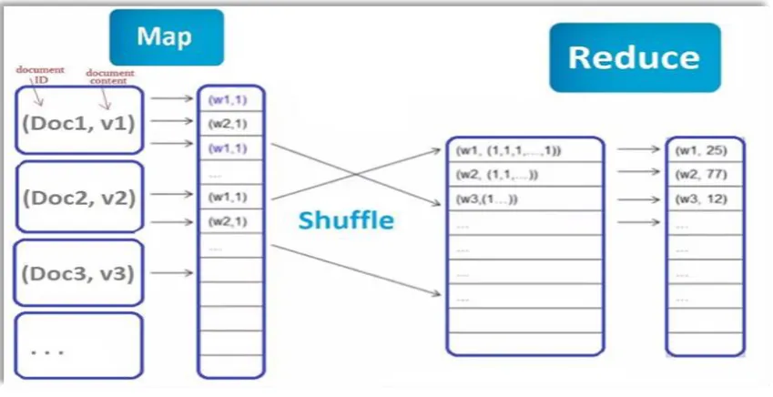
i. Word Count Example:
MapReduce will be explained using a word count example shown in figure 2-5. The
example assumes a collection of documents files Doc1, Doc2, Doc3, and each document
[image:30.595.91.516.192.410.2]has a textual content v1, v2, v3, respectively.
Figure 2-5: MapReduce word count Example
Initially the file is stored in the HDFS file system in chunks, (see Figure 2-6), where in this case each chunk is one document “Doc”, and each chunk of data is passed to the Mapper.
In the map phase the map function (mapper) will divide the content of each document into words and emit a key-value message that has the word as a key and number 1 as a value
21
Figure 2-6: Map task and Reduce task in Hadoop
In the shuffling phase, the output from the mapper will be aggregated and sorted and all the
messages that share the same key (which is the word here) will be sent to the same reducer.
The intermediate results are stored locally (not in HDFS) as temporary files and then passed
to the reducer.
In the reduce phase, the reducer will receive messages that each has a pair of a words and a
list of values. In this case the reducer will sum all the values for each word to count the
words. The output is stored in the HDFS. The pseudocode for word count example is shown
in figure 2-7.
22
ii. MapReduce Alternatives
a) MapReduce Limitations
MapReduce is one of the most used paradigms for processing distributed file systems.
MapReduce is very flexible as there is no schema or index, however this may give poor
performance when compared to relational databases[55]. For low-latency processing
systems it is not suitable as MapReduce computation uses batch processing unlike the
stream computation which has continuous jobs[55]. Furthermore, much development is
addressing the way it is implemented, as it is not efficient when applications require repeated
MapReduce iterations. This is because MapReduce has no memory since it assumes the input
is too large to fit in memory, and at each iteration it writes to three replicas in the distributed
file system which is an overhead, The map tasks for subsequent iterations cannot begin until
all the previous stages are complete [56]. Improving the performance of MapReduce and
enhancing large-scale data processing have become a very important area of research, with
MapReduce parallel programming being applied to many data mining algorithms [57].
b) MapReduce Evolution
Rajaraman & Ullman [51] identified three approaches to improve the performance of
MapReduce:
Iterate MapReduce: enhance iterated MapReduce run-time and make it more efficient by avoiding the data copy between each iteration and pipelining the output of the reducer
directly into the map phase of the next MapReduce iteration. This approach has been
added to Hadoop as an extension to support iterative algorithms. For example:
o Twister [58], is an iterative MapReduce framework that provides a long
running Map and Reduce tasks the “do not terminate after the execution of
each iteration” capability It also differentiates between two types of data:
23
in each iteration (usually it is the larger of the two). The mapper in Twister
will stream its output directly to the reducer[59].
o HaLoop [60], extends the Hadoop MapReduce framework by supporting
iterative MapReduce applications, adding various data caching mechanisms
and making the task scheduler loop-aware.
o Tez [61] is a project is aimed at building an application framework which
allows for a complex directed-acyclic-graph of tasks for processing data
which allow for dynamic performance optimizations[61]. It enables a user to
run interactive jobs on the top of YARN.
Generalize data-flow graph of MapReduce tasks. This generalizes the MapReduce
paradigm to a system that supports any acyclic collection of functions, where map and
reduce are simply two types of operations, each one can be instantiated by many tasks.
Each is responsible for executing that function on a portion of the data. Examples of
such data flow systems are: DryadLINQ[62],Naiad [44], Hyracks [63], Clustera [64].
o Spark [23], [24], is a framework that supports iterative applications, it
focuses on caching the data between different MapReduce-like task
executions by introducing resilient distributed datasets (RDDs) that can be
explicitly kept in memory across the machines in the cluster.
o Naiad[44], is a Microsoft system for data-parallel dataflow computation that
focusses on low-latency streaming and cyclic computations.
o Stratosphere[65], is an open-source software stack for analyzing Big Data.
Stratosphere recently became an Apache project under the name Apache
Flink[66]. it tries to bridge the gap and combine the flexibility of MapReduce
and the efficiency of parallel DBMSs. It exploits in-memory data streaming
24
introduces special kinds of iterations (delta-iterations) that can significantly
reduce the amount of computation as iterations proceed.
Direct Implementation of recursion in MapReduce [56] to try to solve the problem of
recovering from non-blocking tasks failing, without the need to restart failed tasks. There
are two main models:
o Graph based models such as Pregel [46] and Giraph[67], by using the Bulk Synchronous Parallel (BSP) paradigm, which is considered more efficient
than MapReduce for graph processing. However, it places a restriction of
needing to have a combined memory size of the machines processing the
graph larger than the graph size.
25
2.2.2
Apache Spark
Apache Spark [23], [24] is a fast and general-purpose cluster computing system which has
in-memory nature, It provides similar scalability and fault tolerance properties to
MapReduce using high-level APIs in Java, Scala, Python, and R that enable interactively
querying big dataset on clusters. In addition, it supports a set of tools including Spark SQL
for SQL and structured data processing, MLlib for machine learning, GraphX for graph
processing, and Spark Streaming (shown in figure 2-8).
Figure 2-8: Apache Spark5.
Spark evaluation shows a performance which is up to 20 times faster than Hadoop for
iterative applications, speeds up a real-world data analytics report by 40 times, and can be
used interactively to scan a 1 TB dataset with 5–7 seconds latency[68].
The main abstraction Spark provides, is a Resilient Distributed Dataset (RDD)[69], which
is a read only collection of elements partitioned across the nodes of the cluster that can be
operated on in parallel and can be rebuilt if a node is lost. In addition, it provides two shared
variables:
(1) Broadcast variables, which only copied to each worker once and cache values in memory,
26
(2) Accumulators, in which workers can only add to using an associative operation such as counters and sums.
In Spark, developer writes a driver program that connects to a cluster of workers. In the
driver program one or more RDDs are defined through transformations (e.g., map and filter)
which are lazy operations create a new dataset from an existing one, then action operations
are invoked (e.g., count, collect, save) to run the computation on the dataset and return a
value to the driver (figure 2-9).
Figure 2-9: RDD Operations6
This design increases the efficiency of Spark as transformations are lazy and are only
computed when the first time an action is used to return a value to the driver program. In
addition, Spark can persist an RDD in memory and keep the elements around on the cluster
for much faster access the next time it will be needed. Persisting can be on disk in case we
want to save memory and we don’t want a heavy processing operation to be recomputed.
Figure 2-10:Spark System[69]
6 https://spark.apache.org/docs/latest/rdd-programming-guide.html
Block 1
Block 2
Block 3
Worker
Worker
Worker
Driver
Tasks
Results Cache 1
Cache 2
27
Which could be significantly efficient in applications that need iterative algorithms and
interactive data mining tools (figure 2-10).
As mentioned before RDDs [69] [23] is the main abstraction Spark used to perform
in-memory computations on large clusters where RDD’s elements are partitioned. RDDs
created in transformation operation in four ways:
From a file in a shared file system
By “parallelizing” a Scala collection
By transforming an existing RDD.
By changing the persistence of an existing RDD, either by keeping it in memory or
writing it to a disk.
When an action operation is invoked (e.g., count, collect, save) on RDD, Spark will build a
directed acyclic graph (DAG) of stages to execute based on RDD’s lineage graph. RDD has
enough information about how to compute its partitions from data in stable storage it does
not need to exist on a physical storage and achieves fault tolerance using a notion of lineage
rather than the actual data, thus when data on a partition is lost it will automatically recovered
just on that partition using the transformations that originally created it. In addition, RDD
can be cached or persisted on the cluster for later reuse.
There are three options for storage of persistent RDDs:
in-memory storage as deserialized Java objects,
in-memory storage as serialized data,
28
Internally, RDD interface are represented using five pieces: a list of partitions; preferred
location of a partition; dependencies on parent RDDs; a function to compute based on its
parents; metadata about how the RDD is partitioned. Two kinds of dependencies are
distinguished between RDDs: narrow dependencies, where parent RDD is transformed to
only on child RDD; wide dependencies, where multiple child partitions may depend on it.
Knowing the type of dependencies in RDD helps to make efficient decision to recover a
node failure, as with a narrow dependency only the lost parent partitions need to be
recomputed (figure 2-11).
join with inputs not co-partitioned union
groupByKey
join with inputs co-partitioned map, filter
[image:38.595.98.473.350.674.2]“Narrow” dependencies: “Wide” (shuffle) dependencies:
29
Spark use RDDs to perform in-memory computations on large clusters, similarly to what
Distributed Shared Memory (DSM ) do. However, RDD has many advantage over DSM
such as: DSMs use checkpoint to roll back the whole program upon failure. On the other
hand, RDDs can be recomputed in parallel on different nodes using lineage. Spark can detect
slow nodes and use RDDs to run backup copies on different nodes. When RDDs does not fit
in memory can be stored on disk in a similar way to MapReduce.
RDDs evaluated and used to express a number of other cluster programming frameworks
and help to optimise performance by caching wanted data in memory, partitioning it to
minimize communication, and providing efficient fault tolerance. For example, Spark can
express MapReduce model using flatMap and groupByKey operations, or reduceByKey if there is a combiner. Furthermore, RDDs can be persisted in memory to simply and efficiently
implement Iterative MapReduce model such as HaLoop[60] and Twister[58] through a
series of MapReduce jobs to loop[69].
Currently Spark is one of the most widely used open source processing engines for big data.
It provides rich language-integrated APIs with a wide range of libraries, and both the
30
Chapter 3:
Literature Review:
3.1
Graphs
3.1.1
Introduction to Network
Over the past decade the way we live and work has enormously changed due to the boost
advances in technologies and the increase in complexity of the communication systems
available, this has been reflected mainly in how we become dependent on such technologies
and systems. Moreover, it was predicted that this trend will continue according to the
Gartner’s report “Top 10 strategy technology trends for 2015”[2], which shows that there
has been an increase in adoption and investment in new concepts such as Internet of Things
(IoT), where billions of everyday devices or equipment will be connected to the Internet
using smart machines where smart technologies and devices are evolving rapidly. In another
word, our real world is merging with the virtual world by going beyond many of the
geographic limitations and especially with the increased interactions with social network
systems. In addition, our environment is becoming more intelligent, with the mass volume
of data generated; analytics is now deeply embedded everywhere seeking for a better and
smarter understanding.
With the huge amount of data collected, there is an urgent need to efficiently deal with it and
extract knowledge that no one has discovered before. One approach is to look at this data as
a network with links connecting things together, those links can take different kind of forms
of relationships. This metaphor of networks is currently used in many areas: computer
science, economics, sociology, biology, and many more. It can effectively address many of
the challenges in each area by understanding the “connectedness” of these complex systems.
31
structure - who is connected to whom, and (2) Game Theory: the study of strategic behaviour in the network - by understanding each individual action in correlation with everyone in the
systems and how the system will react to this action [6].
3.1.2
Graph Theory:
Modelling the relationship in a network by graphs helps to generate a natural human
interpretation and simple mechanical analysis [10]. This concept is not new, back few
centuries in 1736 Leonhard Euler in his paper on the Seven Bridges of Königsberg laid the
foundation of graph theory. Since then mathematicians extensively studied graph and its
properties [71].
Almost anything can be represented as a graph [7], if a system contains many single units
interacting with each other through a certain kind of relationship, each node of the graph
stands for one of the units of the system and relationships between different units are
indicated by edges[72]. Graph are considered to be a very flexible data model that can be
used to express relationships between entities, and to recognize local and global
characteristics of the system, and to analyse different features of the complex networks
[8][7][9].
Graphs have been used to understand complex human and natural phenomena [73]. In
general, graph is used in any domain when there is a need to find a network representation
of logical or physical links between entities. Its applications spread on wide variety of
domains such as: linguistics, economics, sociology, biology, chemistry, and pharmacology
(e.g. graphs model the complicated structure of chemical compounds and protein structures),
and computer science (e.g. Worldwide Web, workflows, XML documents, computer
32
networks) and many more, where graph algorithms have been developed to solve different
kinds of problems [7] [8] [74] [75].
3.1.3
Definition
With the diversity of data acquired nowadays, a need to find a way to deal with data beyond
the multi-dimensional model used in traditional database. Graph is way to represent
structured and heterogeneous data as set of objects that are linked to each other in different
ways. A Graph G = (V, E) is consists of set of nodes V (Vertices) that are connected with
each other by links called edges E. Usually Graph represented as directed, undirected graphs,
with weighted edges and nodes, tree graphs, and in many variants. It's used to help studying
the relationship between objects such as paths, positions, associations, sequences and
structures[8] [6] [11].
3.1.4
Characteristics
According to the survey conducted by IBM [8], many graph techniques and algorithms has
been developed showing how data is represented, interoperated and analysed. Usually graph
algorithms categorised as follow:
1. Structural algorithms (network analysis algorithms), that try to understand the
structure of the network and analyse the relationships between network entities and
explore topological properties of a graph, such properties as:
a) Order and Size: the number of nodes and edges.
b) Degree: the number of edges incident for the node, in-degree which is the number
of incident on the node, out-degree which is the number of incident from the
node.
33
d) Diameter: the longest of all shortest paths between two nodes.
e) Girth: the length of the shortest cycle.
f) Connectivity coefficients: the minimum number of nodes that when removed the
graph will be disconnected.
g) Clustering coefficients: a measure to show how nodes cluster together.
h) Centrality: which determines the importance of a node in a graph. The four main
measures of centrality are:
1) Degree Centrality: the degree for that node normalized with the total
number of edges.
2) Closeness Centrality: is a measure for distance between a node and all
other nodes in the graph.
3) Betweenness Centrality: is a measure for the number of shortest paths go
through a node divided by the number of shortest path in the graph.
4) Eigenvector Centrality: is a measure for the importance of a node in the
graph.
2. Traversal algorithms, which navigate paths in a graph to solve problems such as: (a)
route problems by trying to optimize path lengths under certain conditions. (b) Flow problems, for example, investigate flow of oil or gas over a directed graph. (c)
Coloring problems as partition the graph by labelling its entities. (d) Searching problems by traversing nodes to answer query or find a problem stated.
3. Pattern-matching algorithms, by finding different graph patterns (e.g., cliques,
cycles, sub-graphs, network motifs) in a graph. Interesting application for this type
of algorithms include: social analytics, organizational analytics, epidemiology,
34
Applying the mining algorithms on graph data is a challenge, as the graph miners need to
adapt or redesign their algorithms to be able to handle the new measures and properties of
graphs and be able to store, query and explore graphs in a similar way as in traditional
databases. Because of the fact that the structure of data is different, it hard to defined graph
measures and properties using classical data mining algorithms. In addition to the fact that
usually recent graphs are very big and does not fit in memory to be handled using traditional
mining algorithms[11] .
3.2
Big Graph
According to Skhiri [11], nowadays there is an urgent need to deal with structured,
unstructured, and heterogeneous data instead of the traditional one. Thus, graphs are now
widely used because of its expressive power and the ability to connected object in different
way. However, mining is hard to implement because of the structure of the data, and size of
the data as the real-world graphs are very big, and usually does not fit in a machine memory.
Adding to that, there is no single model that efficiently fits all the types of graph algorithms
and application, nonetheless many have been developed to solve specific problems or to
meet some special classes of applications.
3.2.1
Big graph History:
Graph processing is not new, it is a well-investigated area of research, in addition big graph
has been always a problem. However, the perception of defining how large is big graph has
been evolving.
35
was toward using High-performance computing (HPC) using shared memory parallel
systems, which is an active area of research and development.
Nowadays, a rising trend to capture and store any data available, especially as the cost of
storage decreasing and ability to capture different kind of data increase. Pushed by the world
getting more connected; more connected devices and embedded sensors and expanding
networks and others all contribute to found the area of the Internet of Things (IoT); in
addition, people life is more digital nowadays than ever before, and there is increasing
presence of social media in our life (Facebook, Twitter, Snapchat, Instagram, and many
more).
The existing real-world dataset is getting large enormously, these datasets reflect different
kind of relationships and can be generally efficiently represented using graph structures.
However, as the graph grow larger their size and complexity go beyond single processing
machine ability and make processing it with HPC systems a challenging task which is not
always suitable for it[14].
Appearance of the MapReduce concept and its implementation in Hadoop equipped
researchers with a powerful tool to process large graphs, and a new trend toward processing
large graphs in cluster using distributed systems with commodity hardware raised (Scaling out).
It is challenging to ensure the traditional set of properties ACID (Atomicity, Consistency,
Isolation, Durability) in graph database because of the different data structure, as a result,
new tools and data models were developed to adapt to the new data structure. For example,
new querying languages proposed like, Datalog, Xpath, Gremlin, Cypher, SPARQL to
36
Likewise, new techniques for handling large graph processing developed, Skhiri[11]
introduce three categories: (1) high-performance graph DB such as DEX or Titan, (2)
in-memory and HPC/MPI graph processing such as SNAP, and (3) distributed approach based
on Bulk Synchronous Processing (BSP) such as Pregel. Hence Graph Management Systems
(GMS) solutions developed could be categorised as[56], [77]:
a) Transactional GMS such as: Neo4j (centralized graph database), Jena,
HyperGraphDB, RDF3x.
b) Analytic GDM such as Pregel (open source implementation Giraph)
37
3.2.2
Big Graph Systems categorisation
The development in graph processing has recently flourish especially with unprecedented
amount of data acquired and captured, in addition it is motivated and inspired by the latest
advances in big data processing. Pushed by the big data processing move, many systems
have been developed to process, manage and analyse graph data.
We could identify two main categories in the big graph systems:
Graph Databases systems: which is a database founded on the graph structure
(vertices and edges with their properties) to represent the graph data and store it, and
provide the means to query and retrieve data efficiently.
Distributed graph processing systems: which provide the ability to do graph
analytics using iterative processing algorithms in distributed manner on cluster more
efficiently and reliably than the graph database systems can do.
3.2.3
Big graph system requirements:
Junghanns and Guerrieri [76] [78] both indicate that in order to have systems that can
flexibly manage big graphs and can efficiently analyze them the following requirement
should be met:
1. The graph systems should be adaptable with powerful graph model that is not
restricted to fixed schema, but it would be able to process graph with heterogeneous
vertices and edges with different kinds of data and provide tools to process and
analyze it.
2. Provide a powerful query language to retrieve and analyze graph data, and support
38
3. High performance and scalability in graph systems should be offered, to achieve that
in graph databases the emphasis is on how to support query optimization, indexing
and efficient graph storage that can expand as the size of the graph increase. On the
other hand, with distributed graph processing systems, the main focus is on how to
efficiently implement graph operator and partition the large graph in a distributed
cluster, in addition offer expanding processing power when needed by expanding the
cluster by increasing the number of nodes.
4. Providing persistent graph storage and offering support for ACID compliant
transactions on persistent data, reading it, analyze it, and storing it back in distributed
systems.
5. Graph processing system should not offer the user hard and complex experience
when analyzing the data, instead it should offer powerful tool to query the data, in
addition the ability to interactively explore the data and visualize it.
6. Failure is most likely to happen in big clusters and it is very important for the system
to be resilient to failure so the computation will continue even when a node or process
39
3.2.4
Graph databases
Graph databases are used to store data that is based on graph structure with Create, Read,
Update, and Delete (CRUD) methods, they provide graph operators which are designed to
enhance the performance on graph transformation and computation. They are generally
designed to be used with online transactional processing (OLTP) systems, where special
optimizations for performance, integrity, and availability are considered[79].
Usually one or more graph data model is supported in Graph Databases. A graph data model
is the conceptual representation that is used to model the real world entities and the relations
among these entities as a graph[79], [80].
Majority of graph databases support the Property Graph Model (PGM), in which a set of key-value pairs can be associated with any vertex or edge in a directed
multigraph, however only edges with one start vertex and end vertex are permitted.
From the Semantic Web movement comes another graph model Resource Description Framework (RDF), it has in its structure collections of triples (subject-predicate-object), where vertices are (subjects, objects) and edges are (predicates).
These triples form a directed labelled multigraph [76].
Only a few graph database systems use the Generic Graph Model called Hypergraph in which it supports arbitrary user-defined data structures to be attached to vertices
and edges. In contrary to PGM, in hypergraph It is permitted to have edges with any
number of vertices at each end similar to many-to-many relationships in traditional
databases[79]. Such systems provide flexibility to model another graph models, but
also restrict the ability to provide optimized operators for graph transformation and
![Figure 2-11: RDD dependencies[69].](https://thumb-us.123doks.com/thumbv2/123dok_us/8681664.874864/38.595.98.473.350.674/figure-rdd-dependencies.webp)
![Figure 4-4 MemoryCC Algorithm[119].](https://thumb-us.123doks.com/thumbv2/123dok_us/8681664.874864/90.595.87.560.182.589/figure-memorycc-algorithm.webp)