Analysis and Recurrent Computation of MBF of the Maximum Types

(1)

Analysis and Recurrent Computation of MBF of the

Maximum Types

Tkachenco V. G.1,*, Sinyavsky O. V.2

1

Institute of Radio, Television, Electronics, Odessa National Academy of Telecommunications n.a. A.S.Popov, Ukraine

2

Department of Fundamental Sciences, Odessa Military Academy, Ukraine

Abstract

This manuscript is a continuation of the research of monotone Boolean functions (MBF), using the MBF partition into types. An interesting connection is observed between the intersection of the groups of MBF stabilizers of n-1 rank and the number of isomorphic functions of the nth rank. The number of MBFs of the nth rank obtained from the MBF pairs of n-1 rank is computed. The examples of recursive construction of the MBF of the nth rank are shown. The partitioning of the MBF of maximal types into classes is given. The number of classes of functions of the nth rank is computed. A new classification of monotone Boolean function of maximal types into schemes has been developed. Such schemes are given for 3-7 ranks of the MBF. The dependencies between the maximal types of MBF of the nth rank and the n-1 rank are found, which makes it possible to reduce the MBF enumeration by constructing the equivalence classes of the nth rank from the equivalence classes of n-1 rank. The proposed methods are convenient for analyzing large MBF ranks.

Keywords

Monotone Boolean Functions, MBF Types, Maximum Types, MBF Profile, MBF Schemes, MBF Equivalence Classes

1. Introduction

In 1897, R. Dedekind published an article [1], in which the number of elements of a distributive lattice with four generators was found. The number ψ(n) of elements of the distributive lattice with n generators coincides with the number of anti-chains in the unit n-dimensional cube. In the language of the algebra of logic, ψ(n) is the number of monotone Boolean functions depending on the variables x1, ..., xn. The problem of computing ψ(n) is usually called the Dedekind problem. As it turned out, this problem is rather difficult and cannot be solved within the framework of the traditional method of generating functions. There

was an attempt to computation the Dedekind number D(n) through the number of classes of nonisomorphic MBFs. As in the case of D(n), the closed formula for such classes is not known, and in fact only values up to n = 6 were calculated (see [2]). They, apparently, were obtained by a direct method of enumerating all monotone Boolean functions of n variables, and then sorting them into equivalence classes.

In 1997, Engel introduced the concept of a profile of a monotone Boolean function [3]. T. Stephen and T. Yusun [4] parted the whole set of MBF into classes using the profiles, to find the number of nonisomorphic MBF. They developed an algorithm on Matlab to computate the number of classes of such MBFs of 7 variables. This method is based on the partition of the MBF into profiles, which are defined in [3].

Independently the similar MBF concept was introduced by us in work [5]. In [6] classification of MBF on types and enumeration of the MBF maximum types is developed. In [7], a new method for recursively calculating the number Dedekind D(n) was developed on the basis of partitioning into MBF equivalence classes and the algebraic properties of MBF blocks were investigated.

Unlike the profile, the MBF type has an additional digit, with which it is possible to describe all MBFs of a given rank, in particular, the zero MBF. With types it is more convenient to implement an algorithm of computation nonisomorphic MBF equivalence classes. It can be shown that the number of maximal types of MBF n rank equals the number of all types of MBF n-1 rank. Therefore, it is possible to obtain a recurrent formula for calculating equivalence classes and computation the Dedekind number.

(2)

2. Results

The Boolean function of n elements is the mapping h, where . A monotone Boolean function (MBF) is a Boolean function under the condition:

for any such that , then .

The lattice of all MBFs of rank is a free distributive lattice of the rank plus zero MBF (on all sets it is 0) and the unit MBF (on all sets is 1). Under the over / under ratio, we understand the order in this lattice of all MBFs. We will consider the Boolean function in the disjunctive normal form (DNF). MBF can be determined through a DNF. A monotone Boolean function is a Boolean function that does not have a negation operation in the form of a DNF, but only a disjunction and conjunction operation.

A vector is an MBF type if the

i-th component of the vector ai is equal to the number of

conjunctive clauses in the form of DNF, which consist of i variables, i.e. have length i. Several new characteristics were introduced for the type: the number n is called the rank of a type T; the number of non-zero component v – weight of a type T; the number j of the first nonzero components on the right – the right border of the T; the number i of the first nonzero components on the left – the left border of the T; the sum m of all the components of the T – cardinality type T.

The type T is called maximal if, with increasing any of its components by 1, the resulting vector will not be a type, i.e. there is no MBF, the type of which would be equal to this vector. Conversely, if we subtract one or more units from any component, the resulting vector will also be an MBF type, since we will remove the clauses of the length of the corresponding component from the existing MBF. By definition, this function will be monotonic. Thus, any type can be obtained by subtracting integers from components of one or more maximum types.

We call type the

inverse type for type . This means that if the MBF is of type , then the type of disjunctive complement MBF is

Example 1. We take the MBF f from 5 variables equal to one on the input sets 00011, 00111, 01011, 10011, 01111, 10111, 11011, 11100, 11101, 11110 and 11111. The minimal term of the function f are the sets 00011 and 11100, the first of which is at level 3, and the second at level 2 of the Boolean cube. In the symbolic form, the MBF looks like . Hence the type T (f) of f is (0, 0, 1, 1, 0, 0). The rank of this type is n (T) = 5, the weight is v (T) = 2, the left boundary is i (T) = 2, the right boundary is j (T) = 3. The same type has a number of MBFs, in particular MBF with minimal term 00101 and 11001.

Example 2. The following are the maximum types of ranks from 0 to 4.

For rank 0, only type (1) is maximal.

For rank 1, the maximal are 2 types: (0,1) and (1,0). For rank 2, the maximal is 3 types: (0,0,1), (0,2,0) and (1,0,0).

For rank 3, the maximal is 5 types: (0,0,0,1), (0,0,3,0), (0,1,1,0), (0,3,0,0), and (1,0,0,0).

For rank 4, the maximal is 10 types: (0, 0, 0, 0, 1), (0, 0, 0, 4, 0), (0, 0, 1, 2, 0), (0, 0, 3, 1, 0), (0, 0, 6, 0, 0), (0, 1, 0, 1, 0), (0, 1, 3, 0, 0), (0, 2, 1, 0, 0), (0, 4, 0, 0, 0), (1, 0, 0, 0, 0)

We call the types of views

zero, left and right, respectively. For the zero type, the right and left units coincide and are equal to (1).

Let's call a pair of types and rank n admissible if the right boundary of j(T1) is strictly less than the left

boundary of i(T2), i.e. All conjunctive clauses of MBF of

type are strictly less than any clauses of MBF of type .

For any admissible pair of types, a shift-sum operation is defined:

If ,

Such an operation with a zero vector it is possible to carry out both on the right, and at the left:

There are left MBF n-1 rank and right MBF n-1 rank.

Each MBF nth rank of the maximal type consists of an admissible pair of MBFs n-1 rank, left and right connected by separable variable ,

.

It is known that conjunction absorbs conjunction if all its variables are components of conjunction . We say that MBF absorbs MBF , if each conjunction is absorbed by one of conjunction . For the binary representation, it can be written that , i.e. one function is greater than another. This corresponds to the ratio "greater than or equal" on all elements of a free distributive lattice from MBF of rank. From this inequality it follows that and .

Theorem 1. For any admissible pair of maximal types and and any and , we have

.

Proof. In MBF of maximal type contains conjunctions of smaller length than in the second MBF : n

f B →B B=

{ }

0,1

, Bn

α β∈ α β< f

( )

α < f

( )

β

n

(

0, ,..., ,...,1 i n

)

T = a a a a

(

)

1

1 n, n1,..., n i,..., ,1 0

T− = a a− a − a a

(

)

1 0, ,..., ,...,1 i n

T = a a a a

f

T

₁

g

T

11

−

2 1 5 4 3

f

=

x x

∨

x x x

(

0, 0,..., 0 , 1, 0,..., 0 , 0, 0,..., 0,1

) (

)

1

T

T2

1

T

2

T

(

) (

)

(

01 0 2 1 0 11

) (

0 10 1 1

)

, ,..., , ,...,

, ,..., , , ,...,

n n

n n n n

T T T a a a b b b

b a b a ₋ b a c c c₊

= = =

= + + =

 

1 2

T =T T T 1 T21 T11

− ₌ − _ −

(

)

0 0, 0,..., 0

T =

(

) (

)

(

) (

)

1 0 0 1 0 1

0 1 0 1 0 1

, ,..., 0, 0,..., 0 0, ,..., , 0, 0,..., 0 , ,..., ,..., , , 0

n n n

T T T a a a a a a

T T T a a a a a a

− −

= = =

 

1,..., r

f f g1,..., gm

( )

f n

(

1

)

f n−

(

1

)

g n− x_n

( )

(

1

)

n

(

1

)

f n = f n− x ∨g n−

s

t

f g

g f

f ≥g

n

f = ∨f g g= ∧f g

1

T T2 f n1

( )

∈T1 f2

( )

n ∈T2

( )

1 2

f n > f n

( )

1

(3)

by definition of an admissible pair of types. But on the other hand, any conjunction that is added to the maximal is either absorbed by other conjunctions, or is equal to such a conjunction, or itself absorbs one or several conjunctions. But the last two cases cannot be, because we chose the valid types. Consequently, the conjunctions of the first function must absorb the conjunctions of the second function. Therefore . The theorem is proved.

Consequence. If we take the class of isomorphic functions L of type and the class R of isomorphic functions of type from an admissible pair of types, then any function from the first class will be more than any function from the second class.

In any class of isomorphic functions, the permutation maps the MBF to the isomorphic MBF . The product of permutations maps the MBF first

and then , i.e. .

Denote by the action of the group on the MBF . As a result of this action, we obtain a certain orbit of the function , consisting of isomorphic functions that can be transferred from one to another by permutations of this group. The class of all isomorphic MBF n-1 rank, which includes the function , is obtained by acting on of the entire symmetric group .

Suppose there are two classes L and R of isomorphic functions of maximal types n-1 of rank and (see the consequence of Theorem 1). Denote functions of class L , and functions of class R . According to the consequence of the theorem, any pair forms an MBF of the nth rank using an expression

.

In the isomorphic class, the stabilizers of the functions and are connected by such a relation , here is the stabilizer , i.e. groups and are conjugate. In fact,

, Thus, knowing the permutations that takes

to MBF , we can obtain stabilizers for each . It is said that these stabilizers are conjugate to the stabilizer .

Consider stabilizer action on the class R. As a result, we obtain the orbits of cardinality

, respectively. Here .

In particular, we consider the action of on the right MBF , i.e. . The result is an orbit of isomorphic functions . The number of such functions is , here is the stabilizer of the right function . Because if stabilizer is a group, then its action on any of the functions gives the same orbit .

To obtain the orbit , we now take the right function , which not entering into , and we will act on it by the stabilizer . In the same way, we obtain any of the

orbits .

Theorem 2. The number of classes of isomorphic pairs is equal to the number of orbits of the stabilizer of the left (right) MBF n-1 rank acting on the class of isomorphic right (left) MBF. The cardinality of the classes of these isomorphic pairs are proportional to the cardinality of the corresponding orbits.

Proof. We will act using a stabilizer of the left function for a pairs of functions , i.e. . This stabilizer will leave the left function in place, and will transition the right function into orbit . And, obviously, these pairs of functions

will be isomorphic. We map the resulting orbit using a permutation . As a result, we obtain an orbit . Under the mapping , the left function transition to , and the right transition to the set of

isomorphic k functions

,. And, obviously, pairs of

functions will

be isomorphic.

From equality it follows that

. Therefore, this same set of pairs can be obtained by the stabilizer action on a pair of functions

.

Acting so with the others on a pair and combining the obtained pairs of MBF, we obtain the class of isomorphic pairs . Total number of such pairs is

.

Running through all left functions , we obtain an orbit consisting of isomorphic pairs of functions

.

( )

2 f n

( )

1 2

f n > f n

1

T

2

T

p

f p f

( )

s p⋅ f

( )

s f p s f

(

( )

)

(

s p⋅

)( )

f = p s f

(

( )

)

( )

G f G

f

(

1

)

f n−

(

1

)

f n− S_n₋₁

1

T T₂

1,..., r

f f g1,...,gm

(

f g_i, _j

)

( )

(

1

)

_n

(

1

)

f n = f n− x ∨g n−

1

f fi= pi

( )

f1 1

1

i i i

St = p St p− St_i fi

1

St Sti

( )

(

)

( )

(

( )

)

( )

(

)

( )

1 1

1 1 1

i i i i i i i i

i i i

St f p St p f p St p f

p St f p f f

− −

= ⋅ ⋅ = =

= = =

2,..., r

p p

1

f f2,...,fr

2,..., r

f f

1

St

1

St

1,1, 2,1,..., l,1

Or Or Or

1, 2,..., l

k k k k1+k2+ + =... kl m

1

St

1

g St g1

( )

1 Or1,1

1,..., k

i i g g 1 1 1 1 St k St St = ′

 St1′

1

g St1

1,..., k

i i g g 1,1 Or 2,1 Or s

g Or1,1

1

St l

1,1, 2,1,..., l,1

Or Or Or

(

f g_i, _j

)

1

f

(

f g1, 1

)

St1

(

f g1, 1

)

1

f

1

g Or1,1

(

f g1, i1

)

,...,

(

f g1, ik

)

1,1

Or

2

p Or1,2

2

p f1

( )

2 1 2

p f = f

1,..., k

j j

g g

{

}

(

1

)

{

1

}

2 i ,..., ik j,..., jk

p g g = g g

(

f g1, i1

)

,...,

(

f g1, ik

) (

, f g2, j1

)

,...,

(

f g2, jk

)

1 1

i i i

St = p St p−

1

i i i

p St =St p

i St

( )

(

f p gi, i 1

)

i

p

(

f g1, 1

)

(

f g_i, _j

)

1

k r

i f

1

Or k r1

(4)

Then, for the function , we take the right function , which is not in . We will act as before, only instead of a pair of functions we will consider a pair . Also, running through all left functions , we obtain an orbit consisting of isomorphic pairs of functions.

Similarly, we act like this for each orbit , and we obtain all classes of isomorphic pairs of MBFs.

It should be noted that any permutation of a symmetric group translates the left function into one of the functions . And accordingly, the same permutation translates the orbit into one of the orbits . Therefore, there is no way beyond this set of functions. The theorem is proved.

We introduce the concept of an index separating variables . We construct from the MBF n-1 rank, which are the MBF of maximal types of the admissible pair MBF

n rank . A pair of types

is determined uniquely, since this decomposition is unique [8].

If in the same function it is possible to take out other variables outside the brackets, except for and it will not change its appearance, i.e.

, and the functions

and belong to the types that make up an admissible pair, then the number of such variables is called the index of the separating variables .

Theorem 3. The number of MBF n-th rank obtained from pairs of MBF n-1 rank of classes L and R is computed by the formula

Proof. To obtain from the pairs of functions

the class of isomorphic MBFs nth rank is necessary to multiply the left function on the separating variable . The number of functions in the whole class will be equal to the number of pairs multiplied by rank n, since such isomorphic functions are obtained using permutations: (1,2, ..., n), (n, 2,3, ..., n-1,1) etc. Next, you need to divide by the index of separating variables, because functions will be the same. Now the sum over all orbits and obtain the formula . The theorem is proved.

Example 3. Let us find the number of the maximum type of functions of the sixth rank obtained from two isomorphic MBF classes of the maximum type 5th rank. Take the left MBF rank 5, having the type (0,1,6,0,0,0).

The original left MBF

, obtained from the original MBFs permutations

, , ,

functions .

Also right MBF of the 5th rank having type (0,0,0,6,1,0): original MBF

, obtained from the original MBFs permutations

, , ,

functions .

The stabilizer of the first left function includes such permutations.

1. (1,2,3,4,5) 13. (1,4,2,3,5)

2. (1,2,3,5,4) 14. (1,4,2,5,3)

3. (1,2,4,3,5) 15. (1,4,3,2,5)

4. (1,2,4,5,3) 16. (1,4,3,5,2)

5. (1,2,5,3,4) 17. (1,4,5,2,3)

6. (1,2,5,4,3) 18. (1,4,5,3,2)

7. (1,3,2,4,5) 19. (1,5,2,3,4)

8. (1,3,2,5,4) 20. (1,5,2,4,3)

9. (1,3,4,2,5) 21. (1,5,3,2,4)

10. (1,3,4,5,2) 22. (1,5,3,4,2)

11. (1,3,5,2,4) 23. (1,5,4,2,3)

12. (1,3,5,4,2) 24. (1,5,4,3,2)

The same stabilizer and at (so coincided). Now acting on a pair of functions , we obtain the orbit of the first function , which consists of

function.

This orbit will include only one right function . Thus, we have such isomorphic pairs :. Now we map the pair by permutation , i.e. . As a result, we obtain such isomorphic pairs of functions:

and an orbit . Further, on

we will obtain such isomorphic pairs of functions: . Similarly on , we obtain: . Also on obtain: . Now combine the resulting pairs of functions, we obtain a class of 5

isomorphic pairs, orbit:

. The same class of isomorphic pairs of functions can be obtained by choosing the right function and its stabilizer and acting on the left function .

In order to find out the number of MBFs of the sixth rank

1

f gs

1,1

Or

(

f g1, 1

)

(

f g1, s

)

fi

2,i

Or k r₂

j

Or j=1,...,l

n

S f₁

2,..., r

f f

1,1

Or

1,2,..., 1,r

Or Or

λ

( )

(

1

)

_n

(

1

)

f n = f n− x ∨g n−

(

) (

)

(

f n−1 ,g n−1

)

( )

f n

n x

( )

(

1

)

_i

(

1

)

f n = f n− x ∨g n− f n

(

−1

)

(

1

)

g n−

λ

(

f g_i, _j

)

1

l i

i i

k rn K

λ

=

∑

(

f g_i, _j

)

i f

n x

i

λ λ_i

l

1

l i

i i

k rn K

λ

=

∑

( )

1 5 1 2 3 2 4 2 5 3 4 3 5 4 5

f =x ∨x x ∨x x ∨x x ∨x x ∨x x ∨x x

(

)

2 2,1,3, 4,5

p = p₃=

(

3,1, 2, 4,5

)

p₄ =

(

4,1, 2,3,5

)

(

)

5 5,1, 2,3, 4

p = f₂

( )

5 ,...,f₅

( )

5

( )

1 2 3 1 2 4 1 2 5 1 3 4 1 3 5

1 4 5 2 3 4 5

1 5 x x x x x x x x x x x

g x x x x

x x x x x x x

∨ ∨ ∨ ∨ ∨

∨ ∨

=

2 (2,1,3,4,5)

q = q3 =(3,1,2,4,5) q4 =(4,1,2,3,5) 5 (5,1,2,3,4)

q = g2

( )

5 ,...,g5

( )

5

1

St f₁

1

g

1

St

(

f g1, 1

)

1,1

Or

1

1 1

24 1 24 St

k

St St

= = =

′ 

1

g

(

f g1, 1

)

(

f g1, 1

)

p2 p2

(

f g1, 1

)

(

f g2, 2

)

Or1,2:g2 p3

(

f g1, 1

)

(

f g3, 3

)

p4

(

f g1, 1

)

(

f g4, 4

)

5

p

(

f g1, 1

)

(

f g5, 5

)

(

) (

)

{

f g1, 1 , f g2, 2 , f g3, 3 , f g4, 4 , f g5, 5

}

1

g St'1

1

(5)

obtained from pairs of this class, we need to compute the index of the separating variables . Let's make a function of the 6th rank of a pair of functions of the 5th rank , which has the type (0,0,1,12,1,0,0):

,

The same function can be written in another way, taking

out for brackets: , where

, i.e. in this case, the index of separating variables . Therefore, the number of MBFs of the sixth rank obtained from pairs of this class is .

Construct an orbit . To do this, take a function that is not in :

. The stabilizer of this MBF is

1. (1,2,3,4,5) 13. (4,2,1,3,5)

2. (1,2,3,5,4) 14. (4,2,1,5,3)

3. (1,2,4,3,5) 15. (4,2,3,1,5)

4. (1,2,4,5,3) 16. (4,2,3,5,1)

5. (1,2,5,3,4) 17. (4,2,5,1,3)

6. (1,2,5,4,3) 18. (4,2,5,3,1)

7. (3,2,1,4,5) 19. (5,2,1,3,4)

8. (3,2,1,5,4) 20. (5,2,1,4,3)

9. (3,2,4,1,5) 21. (5,2,3,1,4)

10. (3,2,4,5,1) 22. (5,2,3,4,1)

11. (3,2,5,1,4) 23. (5,2,4,1,3)

12. (3,2,5,4,1) 24. (5,2,4,3,1)

Now acting on a pair of functions , we obtain the orbit of the first function , which consists of functions. This orbit will include such right functions: . Thus, we have such

isomorphic pairs: . Now

we will display the same orbit by permutation ,

i.e. . As a result,

we obtain such isomorphic pairs of functions: and an orbit . Further, on we will

receive such isomorphic pairs of functions: . Similarly, on

we get: . Also

on to get: .

Now combine the resulting pairs of functions, we obtain a class of 20 isomorphic pairs:

, , .

In order to find out the number of MBFs of the sixth rank obtained from pairs of this class, we need to calculate the index of the separating variables . Let's make a function of the 6th rank of a pair of functions of the 5th rank , which has the type (0,0,1,12,1,0,0):

,

This function cannot be written so to take out other variable out the brackets, except for , i.e. in this case, the index of separating variables . Therefore, the number of MBF of the sixth rank, obtained from pairs of

this class is .

Therefore, the total number functions of the 6th rank, having the type (0,0,1,12,1,0,0) are .

Theorem 4. The total number classes of functions nth rank obtained from the two classes n-1 of the rank L and R are

Proof. Denote the cardinality of the first stabilizer by . Let the stabilizer have different cardinalities of possible intersections with stabilizers , . We denote the cardinalities of these intersections by . Let the intersection is carried out for functions belonging to the class R. Then there are orbits of cardinality . According to

previously proven . Then .

The theorem is proved.

λ

(

f g1, 1

)

( )

6 1

( )

5 6 1

( )

5

f = f x ∨g

( )

1 6 2 3 6 2 4 6 2 5 6 3 4 6

3 5 6 4 5 6 1 2 3 1 2 4 1 2 5

1 3 4 1 3 5 1 4 5 2 3 4 5

6

f x x x x x x x x x x x x x x

x x x x x x x x x x x x x x x x x x x x x x x x x x x x

∨ ∨ ∨ ∨ ∨

∨ ∨ ∨ ∨ ∨ ∨

∨ ∨ ∨ ∨

=

1

x f

( )

6 = f1

( )

5 x1∨g1

( )

5

( )

1 5 6 2 3 2 4 2 5 3 4 3 5 4 5

f =x ∨x x ∨x x ∨x x ∨x x ∨x x ∨x x 2

λ =

1 1

1 5 6 15 2 k rn λ ⋅ ⋅ = = 2 Or 1,1 Or

( )

1 2 3 1 2 4 1 2 5 2 3 4 2 3 5

2 4 5 1 3 4 5

2 5 x x x x x x x x x x x

g x x x x

x x x x x x x

∨ ∨ ∨ ∨ ∨

∨ ∨

=

(

f g1, 2

)

2,1 Or 1 1 1 24 4 6 St k St St = = = ′ 

2, 3, 4, 5

g g g g

(

f g1, 2

) (

, f g1, 3

) (

, f g1, 4

) (

, f g1, 5

)

2,1 Or 2 p

(

) (

)

{

}

2 1, 2 , 1, 3 , 1, 4 , 1, 5

p f g f g f g f g

(

f g2, 1

) (

, f g2, 3

) (

, f g2, 4

) (

, f g2, 5

)

2,2: 1, 3, 4, 5

Or g g g g p₃ Or2,1

(

f g3, 1

) (

, f g3, 2

) (

, f g3, 4

) (

, f g3, 5

)

p4

2,1

Or

(

f g₄, ₁

) (

, f g₄, ₂

) (

, f g₄, ₃

) (

, f g₄, ₅

)

5

p Or2,1

(

f g5, 1

) (

, f g5, 2

) (

, f g5, 3

) (

, f g5, 4

)

(

) (

)

{

f g1, 2 , f g1, 3 , f g1, 4 , f g1, 5 ,

(

f g3, 1

) (

, f g3, 2

) (

, f g3, 4

) (

, f g3, 5

)

(

f g4, 1

) (

, f g4, 2

) (

, f g4, 3

) (

, f g4, 5

)

(

f g5, 1

) (

, f g5, 2

) (

, f g5, 3

) (

, f g5, 4

)

}

λ

(

f g1, 2

)

( )

6 1

( )

5 6 2

( )

5

f = f x ∨g

( )

1 6 2 3 6 2 4 6 2 5 6 3 4 6

3 5 6 4 5 6 1 2 3 1 2 4 1 2 5

2 3 4 2 3 5 2 4 5 1 3 4 5

6

f x x x x x x x x x x x x x x

x x x x x x x x x x x x x x x x x x x x x x x x x x x x

∨ ∨ ∨ ∨ ∨ ∨ ∨ ∨ ∨ ∨ ∨ ∨ ∨ ∨ ∨ = 6 x 1 λ = 1 1

4 5 6 120 1 k rn λ ⋅ ⋅ = =

15 120+ =135

1 v j j j t w l a = =

∑

1 St

(

n 1 !

)

a

r

−

= St₁ v

'_j

St

1,..., j= m

1,..., v

w w wj

j t j j t w a j a w 1 1 j j St a

w = St St′ 1

(6)

Consequence. The number of classes nth rank, which are comes from two classes n-1 rank, depend only on the intersection of the stabilizers of their functions. Either one stabilizer left MBF with all stabilizers right MBF, or vice versa, one stabilizer right MBF with all stabilizers left MBF.

Example 4. Find the number of classes of functions of the seventh rank. We take the left MBF of the 6th rank,

having the type (0,2,3,1,0,0,0):

. From it 60 isomorphic MBFs are obtained. Its stabilizer consists of permutations: 1. (1,2,3,4,5,6) 2. (1,2,3,4,6,5) 3. (1,2,3,5,4,6) 4. (1,2,3,5,6,4) 5. (1,2,3,6,4,5) 6. (1,2,3,6,5,4) 7. (2,1,3,4,5,6) 8. (2,1,3,4,6,5) 9. (2,1,3,5,4,6) 10. (2,1,3,5,6,4) 11. (2,1,3,6,4,5) 12. (2,1,3,6,5,4)

The same cardinality in the other stabilizers left MBF

Let's take right MBF 6th rank having permissible type (0,0,0,0,1,4,0). From it produces 15 MBF using such permutations: q2 =

(1,2,3,5,4,6), q3 = (1,2,3,6,4,5), q4 = (1,2,4,5,3,6), q5 =

(5,1,2,3,4,6), q6 = (1,2,5,6,3,4), q7 = (1,3,4,5,2,6), q8 =

(1,3,4,6,2,5), q9 = (1,3,5,6,2,4), q10 = (1,4,5,6,2,3), q11 =

(2,3,4,5,1,6), q12 = (2,3,4,6,1,5), q13 = (2,3,5,6,1,4), q14 =

(2,4,5,6,1,3), q15 = (3,4,5,6,1,2). Its stabilizer consists

of permutations:

1. (1,2,3,4,5,6) 25. (3,1,2,4,5,6)

2. (1,2,3,4,6,5) 26. (3,1,2,4,6,5)

3. (1,2,4,3,5,6) 27. (3,1,4,2,5,6)

4. (1,2,4,3,6,5) 28. (3,1,4,2,6,5)

5. (1,3,2,4,5,6) 29. (3,2,1,4,5,6)

6. (1,3,2,4,6,5) 30. (3,2,1,4,6,5)

7. (1,3,4,2,5,6) 31. (3,2,4,1,5,6)

8. (1,3,4,2,6,5) 32. (3,2,4,1,6,5)

9. (1,4,2,3,5,6) 33. (3,4,1,2,5,6)

10. (1,4,2,3,6,5) 34. (3,4,1,2,6,5)

11. (1,4,3,2,5,6) 35. (3,4,2,1,5,6)

12. (1,4,3,2,6,5) 36. (3,4,2,1,6,5)

13. (2,1,3,4,5,6) 37. (4,1,2,3,5,6)

14. (2,1,3,4,6,5) 38. (4,1,2,3,6,5)

15. (2,1,4,3,5,6) 39. (4,1,3,2,5,6)

16. (2,1,4,3,6,5) 40. (4,1,3,2,6,5)

17. (2,3,1,4,5,6) 41. (4,2,1,3,5,6)

18. (2,3,1,4,6,5) 42. (4,2,1,3,6,5)

19. (2,3,4,1,5,6) 43. (4,2,3,1,5,6)

20. (2,3,4,1,6,5) 44. (4,2,3,1,6,5)

21. (2,4,1,3,5,6) 45. (4,3,1,2,5,6)

22. (2,4,1,3,6,5) 46. (4,3,1,2,6,5)

23. (2,4,3,1,5,6) 47. (4,3,2,1,5,6)

24. (2,4,3,1,6,5) 48. (4,3,2,1,6,5)

The same cardinality in the other stabilizers of the right MBFs.

The cardinality of the various intersections with have the values: 2, 4, 6, 12.

The intersection of the stabilizer of the first left MBF with the stabilizer of the right function :

, the cardinality of the orbit (see Theorem 4) . Total of such right functions

, , .

Intersection with the stabilizer of the right function : . Here we have 2 orbits, the cardinality of each orbit . All such right

functions , one orbit : and

another: .

Intersection with the stabilizer of the right function

: , orbit cardinality .

Total of such right functions , .

Intersection with the stabilizer of the right function

: , orbit cardinality .

Total of such right functions , .

Then total number of classes of functions of the seventh

rank are .

Here in all classes the index of the separating variables . Consequently, the number of MBF seventh rank in these classes (see Theorem 3) is 2520, 1260 (2 classes), 840, 420. And the total number of MBF seventh rank, having the type (0,0,2,3,2,4, 0,0) there are 6300.

The distribution of MBFs by classes of isomorphic functions is conveniently presented in the form of diagrams, where we indicate the number of isomorphic MBFs in each class of rank , the number of MBFs in class of rank , which consists of classes of rank . Further, in parentheses the index of separating variables in this class and in square brackets is the number of types for this scheme. Such schemes completely define the number of isomorphic and nonisomorphic MBFs in the type that belongs to this scheme, i.e. all types belonging to this scheme have the same number of isomorphic and nonisomorphic MBF.

Below are the schemes for 3 - 7 ranks. As can be seen from these schemes that, up to the fifth rank, of two classes of rank, only one class of rank is always obtained and either class L or class R consists of only one MBF. This is a scheme of the first type. And starting from the sixth rank there are such types that from two classes of rank consisting of more than one MBF it is possible to form more than one class of rank .

( )

1 6 1 2 3 4 3 5 3 6 4 5 6

f =x ∨x ∨x x ∨x x ∨x x ∨x x x

1

St 6!

12 60

a= =

2,..., 60

St St

( )

1

( )

2 6 ,..., 5 6

g g 1 ' St 6! 48 15= 2 15 ' ,..., ' St St 1 St 1 15 ' ,..., '

St St v=4

1

St

7

' St

1 1 7 2

w = St St′ =

1

12 6 2

a

w = =

1 6

t = g7

( ) ( ) ( )

6 ,g8 6 ,g9 6 g11

( )

6 ,g12

( )

6 ,g13

( )

6

1

St

1

'

St w2 = St1St1′ =4

2

12 3 4

a

w = =

2 6

t = g1

( ) ( ) ( )

6 ,g2 6 ,g3 6

( ) ( ) ( )

4 6 , 5 6 , 6 6

g g g

1

St

10

'

St w3= St1St10′ =6

3

12 2 6 a w = =

3 2

t = g10

( )

6 ,g14

( )

6

1

St

15

'

St w4 = St1St15′ =12

3

12 2 6

a

w = =

4 1

t = g15

( )

6

1

6 2 6 4 2 6 1 12 5

12 12 12 12

v j j j t w l a = ⋅ ⋅ ⋅ ⋅ =

∑

= + + + = 1 λ = 1 n− 1

n− n−1

1 n−

(7)

Table 1. Types of classes MBF 3 rank

No. p/p Cardinality of class Number of classes Number of MBF

1 1 4 4

2 3 1 3

In total 5 7

Schemes of recursive construction of MBF 3 rank 1) 1.1. 1◦1 → 1(3) [4];

2) 1.2. 1◦1 → 3(1) [1].

1 1 5 5

2 4 3 12

3 6 2 12

In total 10 29

2) 1.2. 1◦1 → 4(1) [3]; 3) 1.3. 3◦1 → 6(2) [2].

1 1 6 6

2 5 6 30

3 10 8 80

4 20 2 40

5 30 4 120

In total 26 276

2) 1.2. 1◦1 → 5(1) [6]; 3) 1.3. 4◦1 → 10(2) [6]; 4) 1.4. 4◦1 → 20(1) [2]; 5) 1.5. 6◦1 → 10(3) [2]; 6) 1.6. 6◦1 → 30(1) [4];

1 1 7 7

2 6 10 60

3 15 15 225

4 20 6 120

5 30 8 240

6 60 28 1 680

7 90 4 360

8 120 9 1 080

9 180 18 3 240

10 360 4 1 440

[image:7.595.64.526.62.752.2] [image:7.595.67.529.90.152.2]

(8)

Table 5. Types of MBF partitions of maximum types into classes

No. p/p Cardinality of part. Num. of schemes Number of types Num. of class Num. of MBF

1 1 11 87 87 4 717

2 2 2 5 10 1 335

3 3 1 4 12 2 400

In total 14 96 109 8 452

2) 1.2. 1◦1 → 6(1) [10]; 3) 1.3. 10◦1 → 15(4) [2]; 4) 1.4. 5◦1 → 15(2) [12]; 5) 1.5. 10◦1 → 20(3) [6]; 6) 1.6, 5◦1 → 30(1) [8]; 7) 1.7. 20◦1 → 60(1) [2]; 8) 1.8. 10◦1 → 60(1) [22]; 9) 1.9. 30◦1 → 90(2) [4]; 10) 1.10. 20◦1 → 120(1) [4]; 11) 1.11. 30◦1 → 180(1) [10]; 12) 2.1. 10◦5 → 120(1)+180(1) [4]; 13) 2.2. 5◦5 → 15(2)+120(1) [1];

14) 3.1. 10◦10 → 60(1)+180(1)+360(1) [4].

1 1 8 8

2 7 15 105

3 21 26 546

4 35 18 630

5 42 21 882

6 105 78 8 190

7 140 34 4 760

8 210 79 16 590

9 420 222 93 240

10 630 64 40 320

11 840 96 80 640

12 1 260 290 365 400

13 2 520 172 433 440

14 5 040 28 141 120

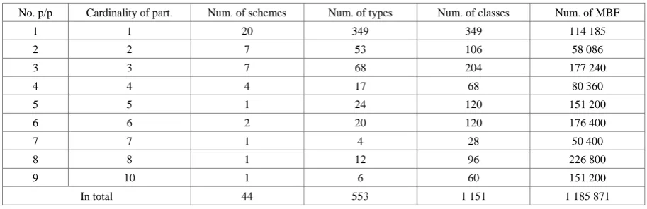
In total 1 151 1 185 871

Table 7. Types of MBF partitions of maximum types into classes

No. p/p Cardinality of part. Num. of schemes Num. of types Num. of classes Num. of MBF

1 1 20 349 349 114 185

2 2 7 53 106 58 086

3 3 7 68 204 177 240

4 4 4 17 68 80 360

5 5 1 24 120 151 200

6 6 2 20 120 176 400

7 7 1 4 28 50 400

8 8 1 12 96 226 800

9 10 1 6 60 151 200

[image:8.595.70.527.368.645.2] [image:8.595.69.526.596.744.2]

(9)

2) 1.2. 1◦1 → 7(1) [15]; 3) 1.3. 15◦1 → 21(5) [2]; 4) 1.4. 6◦1 → 21(2) [20]; 5) 1.5. 20◦1 → 35(4) [6]; 6) 1.6. 15◦1 → 35(3) [12]; 7) 1.7. 6◦1 → 42(1) [20]; 8) 1.8. 30◦1 → 105(2) [8]; 9) 1.9. 15◦1 → 105(1) [48]; 10) 1.10. 60◦1 → 140(3) [2]; 11) 1.11. 20◦1 → 140(1) [22]; 12) 1.12. 90◦1 → 210(3) [4]; 13) 1.13. 60◦1 → 210(2) [22]; 14) 1.14. 30◦1 → 210(1) [20]; 15) 1.15. 120◦1 → 420(2) [4]; 16) 1.16. 60◦1 → 420(1) [72]; 17) 1.17. 180◦1 → 630(2) [10]; 18) 1.18. 90◦1 → 630(1) [14]; 19) 1.19. 120◦1→840 (1) [10]; 20) 1.20.180◦1→1 260(1) [30];

21) 2.1. 6◦6 → 21(2)+210(1) = 231 [4]; 22) 2.2. 6◦6 → 42(1)+210(1) [1];

23) 2.3. 15◦6 → 105(2)+420(1) = 525 [2]; 24) 2.4. 15◦6 → 210(1)+420(1) [16]; 25) 2.5. 20◦6 → 420(1)+420(1) =840 [10]; 26) 2.6. 15◦1+120◦1 →105 (1)+840(1) = 945 [4]; 27) 2.7. 120◦1+180◦1 → 840(1)+1 260(1) = 2 100 [16]; 28) 3.1. 30◦6 → 2·210(1)+840(1) = 1 260 [2];

29) 3.2. 15◦15 → 105(1)+630 (1)+840(1) = 1 575 [16]; 30) 3.3. 20◦15 → 2·420(1)+1 260(1) [18];

31) 3.4. 60◦6 → 210(2)+840(1)+1 260(1) = 2 310[4]; 32) 3.5. 60◦6 → 420(1)+840(1)+1 260(1) [8]; 33) 3.6. 90◦6 → 3·1 260(1) = 3 780 [4];

34) 3.7. 60◦1+180◦1+360·1 → 420(1)+1 260(1)+2 520(1) = 4 200;

35) 4.1. 20◦20 → 2·140(1)+2·1 260(1) = 2 800 [5]; 36) 4.2. 30◦15→210 (1)+ 2·840(1)+ 1 260(1) = 3 150

[4];

37) 4.3. 30◦20 → 2·840(1)+ 2·1 260(1) = 4 200 [2]; 38) 4.4. 180◦6 → 2·1 260(1)+ 2·2 520(1) = 7 560 [6]; 39) 5.1. 60◦15 → 420(1)+840(1)+2·1 260(1)+2 520(1)

= 6 300 [24];

40) 6.1. 60◦20 → 2·420(1)+2·1 260(1)+2·2 520(1) = 8 400 [12];

41) 6.2. 90◦15 → 3·630(1)+3·2 520(1) = 9 450 [8]; 42) 7.1. 90◦20 → 6·1 260(1)+5 040(1) =12 600 [4]; 43) 8.1. 180◦15 → 3·1 260(1)+4·2 520(1)+5 040(1)

=18 900 [12];

44) 10.1. 180◦20 → 4·1 260(1)+4·2 520(1)+2·5 040(1) =25 200 [6].

3. Conclusions

This paper presents a method for partitioning MBF

maximal types into equivalence classes based on MBF of the previous rank. According to the results of this paper, a program was written that finds the number of MBFs of the maximum type up to the eighth rank. For lack of space, the tables and the MBF scheme of the eighth rank and the program will be described in an article devoted to the description of MBF of maximal types of rank 8.

In comparison with the work of [4], where non-equivalent MBFs are calculated directly using profiles, which takes considerable time. Therefore, [4] did not provide calculations for rank 8. And our method uses a different approach - recurrent computation, using MBF types of the previous rank and breaking into equivalence classes, which allows us to obtain a calculation for each type in a split second. This article only considers the maximum types of MBF. For non-maximal types – the subject of further research.

We present the data of the running program for one type (0,0,3,4,0,3,0,0):

Max. type 7 rank #341. (0, 0, 3, 4, 0, 3, 0, 0) is the shift-sum of the maximum types 93. (0, 3, 3, 0, 0, 0, 0) [20 in 1cl] and 8. (0, 0, 0, 1, 0, 3, 0) [20 in 1cl] of rank 6. Weight and cardinality of the selected type is 3 and 10. Left and right borders of the selected type are 2 and 5. This type has 4 equivalence classes of MBFs, which include 2800 MBF. The number of MBFs in each of the equiv. classes equals: 140, 1260, 1260, 140 Ind.part. equal to: 1,1,1,1

Non-isomorphic MBFs from every class that have this type:

140:x x1 7∨x x2 7∨x x3 7∨x x x4 5 7∨x x x4 6 7∨x x x5 6 7∨ 1 2 3 1 2 4 5 6 1 3 4 5 6 2 3 4 5 6

x x x x x x x x x x x x x x x x x x

∨ ∨ ∨ ∨

1260:x x_{1 7}∨x x₂ ₇∨x x_{3 7}∨x x x_{4 5 7}∨x x x₄ ₆ ₇∨x x x_{5 6} ₇∨

1 2 4 1 2 3 5 6 1 3 4 5 6 2 3 4 5 6

x x x

x x x x x

∨

3 4 5 1 2 3 4 6 1 2 3 5 6 1 2 4 5 6

x x x

x x x x x

∨

4 5 6 1 2 3 4 5 1 2 3 4 6 1 2 3 5 6

x x x

x x x x x

∨

Max. types of MBF rank 7 with 4 classes of isomorphic MBFs (17 types): (0,0,0,7,15,1,0,0), (0,0,0,12,4,3,0,0), (0,0,1,2,15,1,0,0), (0,0,1,4,5,4,0,0), (0,0,1,4,7,3,0,0), (0,0,1,4,10,2,0,0), (0,0,1,5,12,1,0,0), (0,0,1,12,5,1,0,0), (0,0,1,15,2,1,0,0), (0,0,1,15,7,0,0,0), (0,0,2,10,4,1,0,0), (0,0,3,0,4,3,0,0), (0,0,3,3,3,3,0,0), (0,0,3,4,0,3,0,0), (0,0,3,4,12,0,0,0), (0,0,3,7,4,1,0,0), (0,0,4,5,4,1,0,0).

Schemes of MBF rank 7 with 4 classes of isomorphic MBFs

4.1. 20◦20 → 2*140(1)+2*1 260(1) = 2 800 2 800 = 2*140+2*1 260 = 2*20*7*1+2*20*7*9 MBFs

Ind.separ.var. equal to 1,…,1(4). Cardinality of the stabilizer 7! /20 = 5 040/20 = 252 5 types

(10)

4.3. 30◦20→ 2*840(1)+ 2*1 260(1) = 4 200 4 200 = 2*840+2*1 260 = 2*30*7*4+2*30*7*6 MBFs

4.4. 180◦6→ 2*1 260(1)+ 2*2 520(1) = 7 560 7 560 = 2*1 260+2*2 520 = 2*180*7*1+2*180*7*2 MBFs

REFERENCES

Dedekind R. Uber Zerlegungen von Zahlen durch ihre [1]

gr ¨ ¨ossten gemainsamen Teilor // Festschrift Hoch. Braunschweig u. ges. Werke. II. — 1897. — S. 103–148. N. J. A. Sloane, The online encyclopedia of integer [2]

sequences, http://oeis.org, 2011.

K. Engel, Sperner theory, Cambridge University Press, [3]

1997.

arXiv:1209.4623v1 [cs.DS] 20 Sep 2012 [4]

Ткаченко В.Г. Классификация монотонных булевых [5]

функций при синтезе цифровых схем / В.Г. Ткаченко // Наукові праці ОНАЗ ім. О.С. Попова. – 2008. – № 1. – С. 35 – 43.

Ткаченко В.Г. Перечисление типов монотонных [6]

булевых функций при синтезе цифровых схем / В.Г. Ткаченко // Наукові праці ОНАЗ ім. О.С. Попова. – 2008. – № 2. – С. 54 – 69.

Tkachenco V.G., Sinyavsky O.V. Algebraic Objects of [7]

MBFs and Recursive Computation of the Dedekind Number, Computer Science and Information Technology Vol. 5(4), pp. 140 – 147 DOI: 10.13189/csit.2017.050404 Tkachenco V. G. Sinyavsky O. V. (2018). Maximum MBF [8]