To Improve the Performance of Secondary Structure Prediction by Soft Computing Technique

(1)

International Journal of Emerging Technology and Advanced Engineering

Website: www.ijetae.com (ISSN 2250-2459,ISO 9001:2008 Certified Journal, Volume 3, Issue 12, December 2013)

414

To Improve the Performance of Secondary Structure Prediction

by Soft Computing Technique

Shivani Agarwal

1

, Sakshi Bhardwaj

2

, Shivangi Gupta

3

1_{Assistant Professor, IMS Engineering College, Ghaziabad.} 2,3_{B.Tech IVth year, C.S.E., IMS Engineering College, Ghaziabad.}

Abstract— Proteins, one of the basic building blocks of all the organisms, need exploratory techniques to predict its complex structures. Machine learning technique such as neural network has been widely used in predicting secondary structures of amino acid sequences. Today, the main aim is to improve the performance of secondary structure predictions by learning a predictive model trained on known structures. Multi-layered feed forward neural network model is trained with the help of hidden layer and by varying sliding window size to determine optimal window size giving highest accuracy. Binary bit encoding scheme is used to encode input training sequence in 3 state DSSP codes. The current efficiency achieved through this technique has reached up to 70% .The experimental results reveal that the following proposed algorithm yields an improved performance with an accuracy of 80%.

Keywords— Protein secondary structure prediction, neural network, sliding window size, binary bit encoding, DSSP codes.

I. INTRODUCTION

Proteins are a class of nitrogenous organic compounds made up of one or more long chains of amino acids and are one of the most basic components in all organisms. On the smallest level, proteins are made up of linear sequences of twenty natural amino acids joined together with the help of peptide or covalent bonds. This forms the Primary structure of proteins. Secondary structure of sequences is formed when linear chain of primary structure begins to twist. In an amino acid chain, each amino acid interacts with other amino acids to form three sub-structures-alpha helix, beta sheets and coils. When amino acids begin to twist and fold even more and form bonds using disulphide bridges a three dimensional structure is formed. This three dimensional structure of a single protein molecule or a polypeptide chain is called tertiary structure. The quaternary structure is the final dimensional structure formed by all the polypeptide chains making up protein. It is composed of two or more sub units of tertiary structures.

A. Biological Neural Network

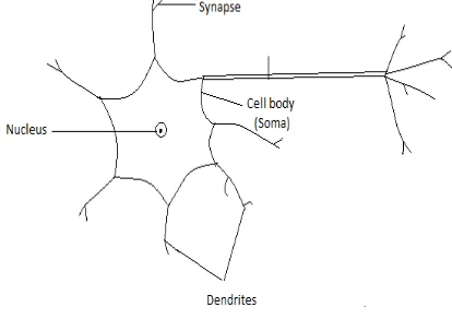
[image:1.612.339.546.402.548.2]

A neuron is a fundamental unit of a neural network. It consists of 3 parts - dendrites, soma and axon. Dendrites are the tree-like structure that receives the electrical signal from the adjacent units, where each line is connected to one neuron. Axon is a single, long connection extending from the cell body and carrying the signals from the neuron. The end of the axon splits into fine strands. At the end of axon, the contact to the dendrites is made through a synapse. It is through synapse that the neuron introduces its signals to the other nearby neurons. A neuron fires an electrical impulse only if certain condition is met. If the sum of the input signals into one neuron surpasses a certain threshold, the neuron transmits this electrical signal along the axon.

Figure 1: Biological Neural Network

B. Artificial Neural Network

(2)

International Journal of Emerging Technology and Advanced Engineering

[image:2.612.84.263.142.302.2]

415

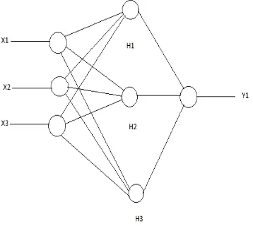
Figure 2: Artificial Neural Network

C. Amino Acids

20 naturally synthesized amino acids have been known. Each amino acid is represented by a basic structure, consisting of a central carbon atom (C), an amino group (NH3) at one end, a carboxyl group (COOH) at the other, and a variable side chain (R), as shown in Figure 3.

Figure 3: Structure of an amino acid

The composition of the side chain determines the shape, the mass, the volume and the chemical properties of an amino acid. 1-letter IUPAC nomenclature for amino acids is widely used in most of the research work.

D. Protein Neural Network Prediction

Training of the specified input signals to the known desired output is facilitated using feed forward neural network which maps the input signals (patterns) to a aspired output. In the secondary structure prediction of neural networks, input is a sliding window with 10-15 residue sequences.

Information from the residues lying in each input window is modified by a weighting factor, summed and sent to a second level, termed as the hidden layer, where the signal on each hidden unit is applied to an activation function to determine the output which is further sent to the output layer representing each of the possible secondary structures [1].The output unit calculate the weighted signal again and sums them, and the signal is applied to the activation function. The output signal is classified into three classes - H (alpha helices), E (beta sheets) and C (coils). Neural network are trained by adjusting the values of the weights that modify signals using a training set of sequences with known structure. The neural network algorithm updates the weight values until the program has been optimized to correctly predict the residues in the training set.

The protein‘s secondary structure prediction- i.e. the prediction of regular local structures such as alpha-helices and beta-strands within a single protein sequence - is an essential intermediate step in predicting the full three-dimensional structure of a protein. If there is knowledge of secondary structure of a protein then it is possible to derive a comparatively small number of possible tertiary (three-dimensional) structures using knowledge about the ways that secondary structural elements associate. We use neural networks to predict protein structures because they are effective. This technique has produced the most accurate secondary structure predictions for the majority of the past decade, starting with [Qian & Sejnowski, 1988].

II. METHODS AND MATERIALS A. Data Set

The Protein Data Bank (PDB [2]) at Brookhaven National Laboratory is a database which contains experimentally determined three-dimensional structures of

proteins, nucleic acids and other biological

macromolecules, with approximately 8000 entries till date. The selection of the data set is taken from Compilation and creation of datasets from Protein Data Bank (ccPDB) source which is datasets generated from the DSSP and PDB Select[3]. The contents, stored as plain text files (in the `PDB' format) are freely accessible and can be downloaded via the websites of its member organizations.

B. Sliding Window Scheme

[image:2.612.58.263.416.535.2]

(3)

International Journal of Emerging Technology and Advanced Engineering

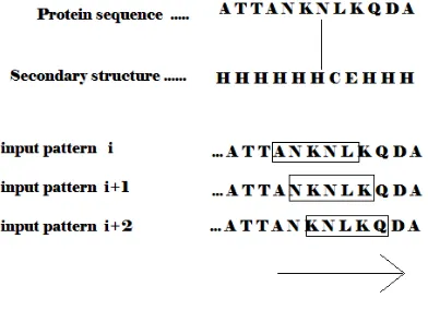
416 In this sliding scheme, a window becomes one training pattern for predicting the structure of the residue at the center of the window in the specified input sequence. Window size training pattern uses the information of the local interactions among neighboring residues. The optimal window length of the sliding window-coding scheme was obtained by experimental analysis of the accuracy of various window sizes on different coding schemes for residues.

Window size should neither be too small nor too large as too small window size may lose relevant and significant Classification information resulting in low prediction accuracy and too large window size includes unnecessary noise.

C. DSSP Codes

The DSSP (Define Secondary Structure of Protein) Algorithm is designed to define the standard method for assigning the secondary structure to the amino acids of a protein. DSSP is commonly used to describe the protein protein secondary structure with single letter codes.

There are eight types of secondary structure that DSSP defines [5]: G = 3-turn helix, H = 4-turn

[image:3.612.63.259.319.461.2]

helix, I = 5-turn helix, T = hydrogen bonded turn , E= extended strand in parallel and/or anti-parallel beta sheet conformation, B = residue in isolated beta bridge, S = bend. Amino acid residues which are not in any of the above conformations are assigned as the eighth type, ‗Coil'.

TABLE I

8-TO-3 STATE REDUCTION METHOD

DSSP Class 8-state symbol

3-state symbol

Class name

310 – helix α- helix π-helix

G H I

H Helix

β-strand E E Sheet

Isolated β bridge Bend

Turn

Rest (connection region)

B S T -

C Loop

D. Binary Bit Encoding Scheme

The feature value of each amino acid residue in the input training pattern is encoded with the help of Binary Bit Encoding Scheme [6]. In this scheme a unique binary

vector to each residue is assigned, such as

(10011),(11000),etc. Here each residue in the training set is encoded with the help of 5 bits. In other words, each residue is assigned a pre-defined binary code ranging from 00000 to 11111.No assigned code should have -all zero or all one bits, four high(1) bits or four low(0) bits in all. This results in 20 possible codes out of 32 possible input codes.

For an example, binary bit encoding for residue A would be (00001), for C-(00010) for D-(00011) for E-(00101) and so on.

III. METHODOLOGY

(4)

International Journal of Emerging Technology and Advanced Engineering

417 The Bias and the weight in the hidden to output layer are not updated and remain the same throughout the whole process. We consider only a single hidden layer so that the time taken for the computations of the results is less and the overall time complexity is less. A binary bit encoding scheme is used in the following algorithm.

Following is our proposed algorithm:

Step 0 to Step 10 describes the training phase of the feed forward neural network and Step 11 to Step 15 explains the testing phase for the network.

Algorithm

Step 0: Initialization and declaration of sequence length (seqn), input sequence (sequence [seqn]), sliding window size (window), learning rate (alpha) and bias (bias).

Step1: Assume random values of hidden layer weights in an array w [][] and output layer weights in an array h[].

Step 2: Provide the target values of input sequence output[i] where i=1 to seqn.

Step 3: Input sequence is encoded using binary bit encoding scheme and stored in an array encode [seqn].

Step 4: For each input to hidden unit,

Calculate net input: hi[i]=hi[i]+(w[j][i]*encode[j])

h[i]= h[i]+bias where i, j=1 to window

Apply activation function on each hidden layer unit.

f(x) = 1/(1+e-x)

activatehi[i]=1/(1+Math.pow(2.718,-1*hi[i]))

Step 5: For output layer, compute the net input:

o=o+ hi[i]*h[i];

where i=1 to window

o=o+ bias

Apply activation function on the output unit.

activation=1/(1+Math.pow(2.718,-1*o))

Step 6: classify into the three classes H, E and C according to the calculated net output response (activation).

O [] =

Step 7: If the output values out[]={H,E,C} do not match the target values output[]={H,E,C} then calculate the error percentage.

erroro= o[i]*(1-o[i])*(t[i]-o[i]) for output unit.

errorh[i]= hi[i]*(1-hi[i])*(erroro*w[i][j]) for each hidden layer unit.

Step 8: Make adjustment in weights and bias for i=1 to window and j=1 to window

w[i][j]= w[i][j]+alpha* erroro *hi[i]

h[i]= h[i]+alpha*errorh[i]

changeb= bias+ alpha*out[i]

Step 9: Test for the stopping condition, i.e., when the final calculated weights of the hidden and output layer in two consecutive passes or epochs are approximately equal or when the final weights become zero.

Else repeat the process again from step 4 till the stopping condition is met.

Step 10: Slide the window by 1 amino acid in the input sequence and repeat the above steps from 1 to 9 till the whole input sequence is trained.

Step 11: Enter the input sequence for which we have a defined PDB output.

Step 12: Give the input sequence in the model.

Step 13: Multiply the input sequence with the weights and the proper steps should be followed to get the output.

Step 14: Classify the output units into three categories H, E and C.

Step 15: Compare the observed output with the already known PDB output and check for errors.

IV. PERFORMANCE MEASURES

The performance of the method for the prediction of secondary structure can be measured in many ways. One of the most commonly used measures is Q3, which is the percentage of correctly predicted residues upon the total observed on three types of secondary structures:

(5)

International Journal of Emerging Technology and Advanced Engineering

418 V. RESULT

On implementation of the proposed algorithm we are recognizing error percentage and increasing accuracy. After all data were collected and transformed to binary bit vectors, weights were assigned to all units of neural network for training and predicting alpha-helix, beta-sheet and combined prediction of both alpha-helix and beta-sheet (three different training sessions) on the training sets taken from PDB. Highest performance on the training set also depends on the number of hidden units. Also, it is analyzed that having more hidden units is not always good it results in high-variance problem. Results reveal that the secondary structure of an amino acid is correlated with that of the neighbourhood sequences, not far from it. This is one of the reasons why we take window to input feature vector.

VI. CONCLUSIONS

The implementation of the above proposed algorithm, the accuracy should come out to be approximately 80%. This gives the conclusion that the multi layered feed forward neural network can be used for the prediction of secondary structure of protein with an accuracy of approximately 80% whereas the highest accuracy with this method till date is 70%.

REFERENCES

[1] Mount, D.W. Bioinformatics: Sequence and Genome Analysis. Cold Spring Harbor Laboratory Press New York (2001).

[2] H M Berman, J Westbrook, Z Feng, G Gilliland, T N Bhat, H Weissig, I N Shindyalov, and P E Bourne. The Protein Data Bank. Nucleic Acids Research, 28:235{242, 2000

[3] Protein Secondary Structure Prediction Using Support Vector Machines, Neural Networks and Genetic Algorithms Anjum B. Reyaz-Ahmed

[4] Hu, H. Yi, P. Improved Secondary Structure Prediction Using Support Vector Machines with a New Encoding Scheme and an Advanced Tertiary Classifier IEEE – Transaction on, Nanobioscience Vol. 3, No. 4 (2004)

[5] G. Pollastri, D. Przybylski, B. Rost and P. Baldi," Improving the Prediction of Protein Secondary Structure in Three and Eight Classes Using Recurrent Neural Networks and Profiles", Department of Information and Computer ScienceInstitute for Genomics and Bioinformatics University of California, Irvine

[6] B. Parvathavarthini, B.Rajesh Kanna and L.Rajeswaridevi, ―Development of Deduced Protein Database Using Variable Bit Binary Encoding.‖ Department of Computer Application, St. Joseph‘s College of Engineering, December 2008.

[7] ―Design of neural network model for analyzing hydrostatic circular recessed bearings with axial piston pump slipper‖. Fazil Canbulut, (Mechanical Engineering Department, Faculty of Engineering, Erciyes University, Kayseri, Turkey.

[8] Soft Computing Methodologies In (Bioinformatics) K.Abraham Computer Science Engineering. V.C.E.T.

[9] http://crdd.osdd.net/raghava/ccpdb/help.html#regsn

[10] Chou, P.Y. ―Prediction of Protein Structure and the Principles of Protein Conformation‖, New York, Plenum Press (1989). [11] ―Protein Secondary Structure Prediction Using Support Vector

Machines, Neural Networks and Genetic Algorithms‖ Anjum B. Reyaz-Ahmed

[12] http://www.theprojectspot.com/tutorial-post/introduction-to-artificial-neural-networks-part-1/7

[13] http://blog.oureducation.in/error-back-propagation-algorithm/