On a Class of Probability Distributions With Application Using Rainfall Data of Kashmir Valley Bilal Ahmad Bhat 1, N. A. Rather2 , T. A. Rather 3

(1)

International Journal of Emerging Technology and Advanced Engineering

Website: www.ijetae.com (ISSN 2250-2459,ISO 9001:2008 Certified Journal, Volume 3, Issue 12, December 2013)

493

On a Class of Probability Distributions With Application Using

Rainfall Data of Kashmir Valley

Bilal Ahmad Bhat

1

, N. A. Rather

2

, T. A. Rather

3

1

Division of Social Science, Faculty of Fisheries, Sher-e-Kashmir University of Agricultural Sciences & Technology of Kashmir, Rangil Ganderbal (J&K) India

2,3_{Department of Mathematics, University of Kashmir, Srinagar-190006 (J&K)}

Abstract—In this paper, we propose a new statistical model

on the pattern of Bilal et al (2010), which yields a class of well-known probability distributions as a special case. Finally, numerical Illustrations using rainfall data of Kashmir valley recorded at Qazigund station has been discussed. It has been observed that Normal distribution is the best fitted model for the annual rainfall data of Kashmir Valley recorded at Qazigund station and can be used for forecasting purpose.

Keywords— Probability density function, Rainfall,

Statistical model, Statistical Software, Kashmir.

I. INTRODUCTION

Statistical models describe a phenomenon in the form of mathematical equations. Thus, a large number of observations say 100 or 1000 can be summarized in an equation with say two unknown quantities (called parameters of the model). Such reduction is certainly necessary for human mind. Out of large number of methods and tools developed so far for analyzing data (on the life sciences etc.), the statistical models are the latest innovations. In the literature (Hogg & Crag (1970), Johnson & Kotz (1970), Lawless (1982) etc.) we come across different types of models e.g., Linear models, Non-linear models, Generalized Non-linear models, Generalized addition models, Analysis of variance models, Stochastic models, Empirical models, Simulation models, Diagnostic models, Operation research models, Catalytic models, Deterministic models, etc. Since the beginning of 1970 attention of the research workers in the discrete distributions appears to be shifted to a new class of discrete distributions known as Lagrangian Distributions. The Lagrangian distributions provide generalization of the classical discrete distributions and thus have been found more general in nature and wider in scope. Consul and Shenton (1972) gave a method for obtaining generalized discrete distributions using the following Lagrange expansion

0 (t))

'

f

(t)

(

1 -s

dt

1 -s

d

1 s

s!

s

U

f(0)

(t)

_























t

g

f

(1.1)

Where f´(t) is the first derivative of f(t). The Lagrangian probability distribution defined on non-negative integers is given by

P ( X = 0) = f(0)

0 (t)

'

f

x

(t))

(

1 -x

dt

1 -x

d

x!

1 x)

(X













t

g

P

; x = 1,2 , …

(1.2) As g(t) and f(t) may be replaced by different sets of p.g.f.s, (1.2) may provide us with families of generalized discrete type of distributions. Some of the important members of this family for some suitably chosen functions g(t) and f(t) are described as under:

Generalized Negative Binomial Distribution

1)

x

-x

(n

x!

x

-x

n

)

-(1

x)

(n

n

x)

(X

















x

P

;

x

-x

n

)

-(1

x

n

x

n









_









 





x

n>0, 0<α < 1, αβ <1, x= 0,1,2,… By taking

)

1 (

1 e

f(t)

and

)

1 (

2 e

g(t)





t







t



Generalized Poisson Distribution

x! ) 2 1 ( 1 ) 2 1 ( 1 x) (X    

 x x e x

P       ;

λ1 > 0,

2 

<1, x = 0,1,2,…

By taking

n

t)

-(1

f(t)

and

t)

-(1

(2)

International Journal of Emerging Technology and Advanced Engineering

494 Generalized Geometric Series Distribution

) 2 x -x ( x! x -x 1 ) -(1 x) (1 x) (X             x P ;

x = 0, 1, 2,… By taking

n

t

f(t)

and

,

m

pt)

(q

g(t)







.

Similarly for suitable choice of g(t) and f(t) a large number of new and well-known distributions can be obtained from (1.2).

Here, our aim is to develop a generalized statistical model on the pattern of Consul (1973), Gupta (1974) etc in case of continuous type of distributions.

II. PROPOSED STATISTICAL MODEL

Let g(x) be a continuous monotonic increasing function in (k,



)

such that g(



)

=



and g(k) =0 where k is any positive real number, then the function

 



 



          _ _ _  x k x g e x g x g x g e x g x g g x f ; ) ( ) ( exp ) ( ) ( ) ( 1 ) ( ) , , , ; (         

=0 elsewhere (2.1) is the pdf of the random variable X of continuous type with

parameters



(



0 )

,



(



0 )

and



(



0 )

.

III. DERIVATION OF WEIBULL DISTRIBUTION

In fact, a number of new and some well-known distributions follow from the model (2.1) for a suitable choice of the function g(x) and the parameters







,

and

. Here we mention only Weibull Distribution

Remark 3.1: Taking g(x)=x so that

g



(

x

)



1

in (2.1), we have

 



 



0 x 0, 0, , ; exp 1 ) (            _           

 _x _x _e x _x _e x

x

f

= 0 elsewhere

Which is the pdf of Modified Weibull Distribution with parameters



(



0 )

,



(



0 )

and



(



0 )

.

Remark 3.2: Taking g(x)=x,

g



(

x

)



1

and





0

in (2.1), we have

  1 exp



 



; 0, 0, x 0 ) (           

  x  x  

x

f

= 0 elsewhere

Which is the pdf of well-known two parameter Weibull distribution with parameters



(



0 )

and



(



0 )

.

Similarly as above, many more distributions can be shown as a particular case of the proposed statistical model (2.1) for a suitable choice of the generating function g(x) and the parameters.

IV. NUMERICAL ILLUSTRATION

(3)

International Journal of Emerging Technology and Advanced Engineering

[image:3.612.65.280.162.442.2]

495

Table 1:

Descriptive Statistics of Annual Rainfall Data (Qazigund Station 1980-2012)

Statistic Value Percentile Value

Sample Size 33 Min 751.7

Range 1133.4 5% 795.17

Mean 1179.3 10% 828.78

Variance 74669.0 25% (Q1) 937.16

Std. Deviation 273.26 50% (Median) 1144.1

Coef. of Variation 0.23171 75% (Q3) 1359.3

Std. Error 47.568 90% 1513.0

Skewness 0.53468 95% 1781.9

Excess Kurtosis 0.04929 Max 1885.1

Table 2:

Results Obtained by Fitting various models to Annual Rainfall Data (Qazigund Station 1980-2012)

S.No. Distribution Parameters

1 Beta 1=1.254 2=2.0976, a=751.7

and b=1885.1

2 Burr k=0.00283 =1332.9 =750.07

3 Burr (4P) k=0.25663 =0.7117 =1.55 =751.7

4 Cauchy =182.08 =1158.2

5 Chi-Squared =1179

6 Chi-Squared (2P) =36024 =-34845.0

7 Dagum k=223.24 =1.7639 =13.594

8 Dagum (4P) k=2.4758 =0.30122,

=0.56895 and =751.7

9 Erlang m=18 =63.315

10 Erlang (3P) m=3 =155.61 =653.5

11 Error k=1.9524 =273.26 =1179.3

12 Error Function h=0.00259

13 Exponential =8.4794E-4

14 Exponential (2P) =0.00234 =751.7

15 Fatigue Life =0.22762 =1149.5

16 Fatigue Life (3P) =0.32694 =802.43 =333.99

[image:3.612.316.568.167.729.2]

(4)

International Journal of Emerging Technology and Advanced Engineering

496

18 Frechet (3P) =7.5688E+7 =1.7260E+10 

=-1.7260E+10

19 Gamma =18.626 =63.315

20 Gamma (3P) =3.379 =155.61 =653.5

21 Gen. Extreme Value k=-0.13096 =250.23 =1063.9

22 Gen. Gamma k=1.0103 =19.203 =63.315

23 Gen. Gamma (4P) k=3.2246 =0.269

=889.91 =751.7

24 Gen. Pareto k=-0.67488 =697.94 =762.61

25 Gumbel Max =213.06 =1056.3

26 Gumbel Min =213.06 =1302.3

27 Hypersecant =273.26 =1179.3

28 Inv. Gaussian =21966.0 =1179.3

29 Inv. Gaussian (3P) =8643.0 =875.18 =304.14

30 Johnson SB =1.5658 =1.7828,

=2418.2 and =440.27

31 Kumaraswamy 1=1.05 2=1.15, a=751.7 and

b=1885.1

32 Laplace =0.00518 =1179.3

33 Levy =1120.5

34 Levy (2P) =234.66 =723.2

35 Log-Gamma =938.51 =0.00751

36 Log-Logistic =7.3169 =1131.8

37 Log-Logistic (3P) =5.7103 =886.48 =260.08

38 Log-Pearson 3 =2130.0 =0.00498 =-3.5693

39 Logistic =150.65 =1179.3

40 Lognormal =0.22652 =7.047

41 Lognormal (3P) =0.29547 =6.7796 =260.88

42 Nakagami m=4.5185 =1.4632E+6

43 Normal =273.26 =1179.3

44 Pareto =2.3546 =751.7

45 Pareto 2 =144.7 =1.9021E+5

46 Pearson 5 =19.778 =22162.0

47 Pearson 5 (3P) =24.717 =31160.0 =-134.08

48 Pearson 6 1=87.065 2=25.479 =331.63

49 Pearson 6 (4P) 1=17.251 2=31.534,

=1588.2 and =271.15

50 Pert M=1109.8 a=751.7 b=1885.1

51 Power Function =0.43739 a=751.7 b=1885.2

52 Rayleigh =940.97

53 Rayleigh (2P) =398.7 =683.83

(5)

International Journal of Emerging Technology and Advanced Engineering

497

55 Rice =1146.3 =273.24

56 Student's t =2

57 Triangular m=901.18 a=751.7 b=1885.1

58 Uniform a=706.03 b=1652.6

59 Weibull =5.1527 =1256.4

[image:5.612.190.547.132.714.2]

60 Weibull (3P) =1.729 =514.55 =719.7

Table 3:

Goodness of Fit – Summary of Rainfall Data (Qazigund Station of Kashmir Valley 1980-2012)

S.N

o. Distribution

Kolmogorov Smirnov

Anderson

Darling Chi-Squared

S

ta

ti

st

ic

Ra

n

k

S

ta

ti

st

ic

Ra

n

k

S

ta

ti

st

ic

Ra

n

k

1 Beta 0.0795 5 1.9507 39 0.5152 8

2 Burr 0.4021 52 53.83 57 N/A

3 Burr (4P) 0.4691 54 13.63 54 N/A

4 Cauchy 0.1341 38 0.8227 34 0.2800 4

5 Chi-Squared 0.3989 51 109.51 58 24.055 48

6

Chi-Squared (2P) 0.0734 3 0.352 18 0.7769 13

7 Dagum 0.8285 58 43.715 56 197.63 52

8 Dagum (4P) 0.5529 56 17.578 55 N/A

9 Erlang 0.1389 40 0.5830 31 0.2756 3

10 Erlang (3P) 0.1859 44 1.3449 36 2.942 37

11 Error 0.0719 2 0.3498 16 0.7027 12

12 Error Function 0.9970 59 284.9 59 41329.0 53

13 Exponential 0.4713 55 9.1871 52 41.029 49

14 Exponential (2P) 0.1884 45 3.4811 43 4.0053 43

15 Fatigue Life 0.1029 18 0.3158 10 0.8226 18

16 Fatigue Life (3P) 0.1122 30 0.3552 20 1.6543 33

17 Frechet 0.1518

8 42 0.7757 33 3.1806 39

18 Frechet (3P) 0.1111 27 0.3614 22 1.6513 32

19 Gamma 0.0903 7 0.2768 3 0.3799 5

20 Gamma (3P) 0.1151 33 0.3696 24 0.89282 20

21 Gen. Extreme V

alue 0.0913 9 0.2704 2 0.4959 7

22 Gen. Gamma 0.0933 12 0.3019 5 0.4539 6

23 Gen. Gamma (4

P) 0.1138 32 4.3588 47 N/A

24 Gen. Pareto 0.0923 10 4.1218 45 N/A

25 Gumbel Max 0.1242 35 0.5093 29 1.4814 28

26 Gumbel Min 0.1365 39 1.3556 37 3.5275 40

27 Hypersecant 0.1080 22 0.5906 32 1.9153 35

(6)

International Journal of Emerging Technology and Advanced Engineering

498

29 Inv. Gaussian (3

P) 0.1117 28 0.3529 19 1.6322 31

30 Johnson SB 0.0905 8 0.2543 1 0.6562 10

31 Kumaraswamy 0.2424 47 3.4017 42 1.9697 36

32 Laplace 0.1302 36 0.9292 35 4.2921 44

33 Levy 0.5593 57 12.991 53 75.764 51

34 Levy (2P) 0.3479 50 4.4822 48 16.83 47

35 Log-Gamma 0.1036 19 0.3101 8 0.8408 19

36 Log-Logistic 0.1309 37 0.4399 26 0.9592 25

37

Log-Logistic (3P) 0.1105 25 0.3979 25 0.91804 23

38 Log-Pearson 3 0.1027 17 0.3069 6 0.8225 17

39 Logistic 0.0928 11 0.4464 27 0.7983 15

40 Lognormal 0.1039 20 0.3208 11 0.8183 16

41 Lognormal (3P) 0.1106 26 0.3488 15 1.5683 29

42 Nakagami 0.0781 4 0.2798 4 0.1760 2

43 Normal 0.0703 1 0.3459 14 0.7023 11

44 Pareto 0.2284 46 4.6554 49 3.8795 42

45 Pareto 2 0.4349 53 8.2339 51 50.673 50

46 Pearson 5 0.1124 31 0.3612 21 1.5794 30

47 Pearson 5 (3P) 0.1093 24 0.3436 13 0.9238 24

48 Pearson 6 0.1092 23 0.3412 12 0.9155 22

49 Pearson 6 (4P) 0.1212 34 0.3645 23 1.4021 27

50 Pert 0.1408 41 3.0958 41 3.8182 41

51 Power Function 0.2641 48 4.1477 46 7.0905 45

52 Rayleigh 0.2817 49 3.9846 44 12.604 46

53 Rayleigh (2P) 0.0944 13 0.3102 9 1.1754 26

54 Reciprocal 0.1778 43 1.7922 38 3.0 38

55 Rice 0.0888 6 0.3516 17 0.0473 1

56 Student's t 1.0 60 446.46 60 4.2257

E+7 54

57 Triangular 0.0998 15 2.2225 40 0.7879 14

58 Uniform 0.1119 29 7.7746 50 N/A

59 Weibull 0.0946 14 0.5409 30 0.5158 9

60 Weibull (3P) 0.1055 21 0.3089 7 0.8990 21

Probability Density Function

Histogram Normal

x

1500 1000

f(

x

)

0.25

0.2

0.15

0.1

0.05

[image:6.612.317.571.133.690.2]

0

(7)

International Journal of Emerging Technology and Advanced Engineering

499 Probability Density Function

Histogram Chi-Squared (2P)

x

1500 1000

f(

x

)

0.25

0.2

0.15

0.1

0.05

[image:7.612.65.274.141.334.2]

0

Figure 3: Fitting of Chi-Square Distribution

Probability Density Function

Histogram Error

x

1500 1000

f(

x

)

0.25

0.2

0.15

0.1

0.05

0

Figure 4: Fitting of Error Distribution

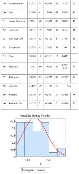
For our data Kolmogorov Smirnov, Anderson-darling and Chi-square test were used for testing the goodness of fit (as shown in Table 3). It seems that Normal, distribution is the best fitted model on the basis of Kolmogorov Smirnov test and can be used for forecasting purpose. Fitting of various distribution is also represented graphically (Figure 2-4). Forecasting rainfall is important as it would enable scientists working in different fields to plan and prepare their activities in an optimal way. From the data (Figure 1) it is observed that rainfall has generally decreased over the years and obviously it is not a stationary time series.

REFERENCES

[1 ] Bhat Bilal A., Raja T.A., Pukhta, M.S. and Agnihotri R.K. 2010.

On a Class of Continuous Type Probability Distributions with Application, Int. J. Agricult. Stat. Sci., Vol.6, N0.1, pp. 147-156.

[2 ] Bhat Bilal A., Raja T.A. and Akhter R. 2008. Statistical Models and

their Applications to Meteorology, Sci. for Better Tomorrow, pp. 393-402.

[3 ] Consul, P.C. 1981. Relation of Modified Power Series Distributions

to Lagrangian Probability Distributions. Comm, Stat. Theor. Meth. A10(20), 2039-2046.

[4 ] Consul, P.C. and Shenton, L.R. 1973b. On the Probabilistic

Structure and Properties of Discrete Lagrangian Distributions. A Modern Course on Statistical Distributions in Scientific Work, D. Riedal Publishing.

[5 ] Consul, P.C. and Shenton, L.R. 1973. Some interesting properties of

Lagrangian distributions, Comm., Stat. 2(3), pp. 263-272.

[6 ] Consul, P.C. and Shenton, L.R. 1972. Use of Lagrangian expansion

for generating generalized Probability distribution, SIAM, J. Applied Math., Vol. 23, No. 2, pp. 239- 248.

[7 ] Draper, N. R. and Smith, H. 1982. Applied Regression analysis,

second Edition. John Willey and Sons, New York.

[8 ] Fawzia, I, Moursy 2000. Trend and Predictions of rainfall over

North Africa, Mausam, 51, 155-162.

[9 ] Gupta, R.C. 1974. Modified Power Series Distribution and Its

Applications. Sankhya, Ser. B, Vol. 36, No.3, pp. 288-298.

[10 ]Hogg, R.V. and Craig, A.T. 1970. Introduction to Mathematical

Statistics, fourth edition, New York: Macmillan.

[11 ]Johnson, N.L. and Kotz, S. 1970. Continuous Univariate

Distributions, Vol 1 and Vol 2, Houghton Mifflin Company, Boston.

[12 ]Kane R.P. 2002. Trends and Predictions and ENSO relationship of

New Zealand rainfall, Mausam, 53, 9-18.

[13 ]Lawless, J.F. 1982. Statistical Models and Methods for Life-Time

[image:7.612.90.271.365.554.2]