Energy efficient Localization Technique in Wireless Sensor Network

(1)

International Journal of Emerging Technology and Advanced Engineering

Website: www.ijetae.com (ISSN 2250-2459,ISO 9001:2008 Certified Journal, Volume 3, Issue 11, November 2013)

148

Energy efficient Localization Technique in Wireless Sensor

Network

K. Padmanabhan

1

, Dr. P. Kamalakkannan

2

, Dr. S. P. Shantharajah

3 1

Asst.Professor, MCE, Tamilnadu, India

2_{Asst.Professor, Govt. Arts College (Autonomous), Salem, Tamilnadu, India} 3_{Professor, Sona College of Technology, Salem, Tamilnadu, India}

Abstract

-

Localization is one of the essential problems in wireless sensor networks (WSNs), since the locations of the sensor nodes are significant to both network operations and application level tasks. Although the Global Positioning System based localization techniques can be used to determine node locations within a few meters, the cost of Global Positioning System devices and non-availability of Global Positioning System signals in limited environments avoid their utilization in large scale sensor networks. There exists an extensive body of research that aims at obtaining locations as well as spatial associations of nodes in wireless sensor networks without requiring specific hardware or employing only a limited number of anchors that are aware of their own locations. In this paper, we propose an anchor free localization technique for single hop WSN. The simulation result shows that the proposed technique outperforms its comparatives.

Keywords - Sensor localization, Wireless sensor networks, Range measurements, Anchors.

I. INTRODUCTION

Wireless sensor networks (WSNs) have many applications that consist of object tracking, traffic monitoring, habitat monitoring, measuring radiation levels from nuclear reactors, detecting seismic activities, navigating ships, and so on. In all these applications, sensor node locations are significant not only to the application’s goals but also for the operations of Wireless sensor networks [1]. An essential problem with the deployment of Wireless sensor networks is the coverage. A coverage technique of sensor nodes would depend on the distance between the point of interest and the nearby node. As a result, locations of sensor nodes from the basic input for the algorithms that observe coverage of the network. Location-based routing (LR) protocols are Location-based on the location information of sensor nodes. The advantages of LR protocols include enhanced scalability and less overhead caused by dynamic changes in topology. Furthermore, location aided routing utilizes location information to find a much smaller request region than the probable searching region for routing paths.

A recent study indicates that even with the help of a simple anchor-free localization algorithm, the LAR protocol performs as competitively as the shortest path routing algorithm under ideal assumptions [2]. Besides, geographic addressing uses the physical locations of nodes as global references to make possible identification and communication in a network. Beyond the networking protocols, the applications involving wireless sensor networks use location information to understand the significance of sensory information from different regions. For example, location information constitutes an important element for analysis about contexts, particularly in smart environments. This paper proposed an anchor free localization method for single hop wireless sensor network. The proposed method is based on internode distances [3]. The average of the Internode distances is used as main metric to localize the reference node in the proposed method. WSN node localization approaches are typically characterized as either range free or range-based. Most range-free techniques rely on radio connectivity alone and try to map the topology of the communication network to physical coordinates. One might consider such range-free methods as simply extreme cases of range-based approach where the range is estimated relative to the maximum communication range of the radio using a single bit: 1 means within range, 0 means out of range [4]. Nevertheless, range-free techniques are quite inaccurate as the communication range is highly variable and dependent on the environment, due primarily to non line-of sight (LOS) conditions, multipath fading, and hardware/antenna variations. Errors of 50-100% of the radio range are common [5]. The advantages of range-free methods include simplicity and low cost, as no additional hardware is necessary. A representative range-free method is presented in [5].

(2)

International Journal of Emerging Technology and Advanced Engineering

149

Otherwise, the node locations can only be determined relative to one another. The term self localization is sometimes used to indicate that the WSN itself performs the localization of its nodes. For static WSN deployments, one can get around performing self localization. Many times, it is feasible to deploy the sensors in pre surveyed locations. These locations can be established on or before deployment time using external equipment. When higher accuracy is required, for instance, a differential GPS could even be used, since its cost and power requirements are not part of the WSN itself. The goal of many WSN applications is to locate something such as a moving object or source of a signal [7]. Such approaches are often referred to as target localization, source localization, or simply localization.

II. RELATED WORKS

The Self Positioning Algorithm (SPA) for Ad-Hoc wireless networks [8] establishes its local coordinate system by setting itself as the source for every node. Two more nodes are arbitrarily selected such that all the three nodes do not lie on the same line to minimize triangulation error and can communicate with other nodes. Anchor Free Localization (AFL) technique [10], which has two phases: In the first phase, a heuristic produces an outline which looks like the original design. In the second phase, all the nodes locally balance the solution by adopting the optimization algorithm to make sure that the energy in new location is less than that in the original location. In this approach, localization is dependent on the communication range of nodes and provides better result only when seven or more networks are connected [12]. Localization fault may increase due to unavailability of direct link between nodes and results into an estimation which is multiple of communication radius R, depending on number of hops.

Assumption Based Coordinates (ABC) [9] which uses a cooperative ranging technique for localization. This method localizes one unknown node at a time by making assumptions, compensating the errors through corrections and use of redundant calculations as more and more information becomes available. In ABC, accumulation of errors increases with number of beacon-free node.

Knowledge-based Positioning System (KPS) [13] which is based on pre-configured awareness of probability distribution of configuration. This approach uses configuration point and the probability distribution function. In Configuration point the position of the determined point which is in the cluster, when deploying the nodes. The probability distribution function is obeyed by each group’s nodes after the sensor nodes’ configuration.

In GPS-less low cost outdoor localization [14], overlapping region of nodes to localizes new nodes considering some reference nodes which are already localized. Nodes localized themselves to the centroid of their reference points and localization error depend on separation distance between two adjacent reference nodes and the transmission range of these reference points. A clustering-based approach [15] was proposed for the local coordinate system configuration where an accumulation factor is introduced to standardize the number of master and slave nodes and the level of connectivity between master nodes. Using uniform coordinates, derived a transformation environment between the two Cartesian coordinate systems to efficiently join them into a global coordinate system. Angle of Arrival (AOA) [11] describes the capacity of the nodes to obtain location information.

III. ISSUES IN LOCALIZATION

Resource limitation: Sensor networks are typically quite resource-starved. Nodes have rather weak processors, making large computations infeasible. Moreover, sensor nodes are typically battery powered. This means communication, processing, and sensing actions are all expensive, since they actively reduce the lifespan of the node performing them. Not only sensor networks are typically envisioned on a large scale, with hundreds or thousands of nodes in a typical deployment. This fact has two important consequences: nodes must be cheap to fabricate, and trivially easy to deploy. The designers must actively work to minimize the power cost, hardware cost, and deployment cost of their localization algorithms.

Node concentration: Many localization algorithms are sensitive to node density. For instance, hop count based schemes generally require high node density so that the hop count approximation for distance is accurate. Similarly, algorithms that depend on beacon nodes fail when the beacon density is not high enough in a particular region. Thus, when designing or analyzing an algorithm, it is important to notice the algorithm’s implicit density assumptions, since high node density can sometimes be expensive if not totally infeasible.

(3)

International Journal of Emerging Technology and Advanced Engineering

150

This problem is exacerbated when a sensor network has a non-convex shape: Sensors outside the main convex body of the network can often prove unlocalizable. Even when locations can be found, the results tend to feature disproportionate error.

Ecological obstacles: Environmental obstacles and terrain irregularities can also wreak havoc on localization. Large rocks can occlude line of sight, preventing TDoA ranging, or interfere with radios, introducing error into RSSI ranges and producing incorrect hop count ranges. Indoors, natural features like walls can impede measurements as well. All of these issues are likely to come up in real deployments, so localization systems should be able to cope.

System configuration: Centralized algorithms are designed to run on a central machine with plenty of computational power. Sensor nodes gather environmental data and pass it back to a base station for analysis, after which the computed positions are transported back into the network. Centralized algorithms circumvent the problem of nodes’ computational limitations by accepting the communication cost of moving data back to the base station. This tradeoff becomes less palatable as the network grows larger, however, since it unduly stresses nodes near the base station. Furthermore, it requires that an intelligent base station to be deployed with the nodes, which may not always be possible. In contrast, distributed algorithms are designed to run in the network, using massive parallelism and inter-node communication to compensate for the lack of centralized computing power. Often distributed algorithms use a subset of the data to solve for each position independently yielding an approximation of a corresponding centralized algorithm where all the data is considered and used to solve for all the positions simultaneously.

There are two important approaches to distributed localization. The first group, beacon-based distributed algorithms, typically starts with some group of beacons. Nodes in the network obtain a distance measurement to a few beacons, and then use these measurements to determine their own location. In some algorithms, these newly localized nodes become beacons to help other nodes localize. The second group approaches localization by trying to optimize a global metric over the network in a distributed fashion. This group split out into two substantially different approaches. The first approach, relaxation-based distributed algorithms is to use a coarse algorithm to roughly localize nodes in the network.

This coarse algorithm is followed by a refinement step, which typically involves each node adjusting its position to optimize a local error metric. By doing so, these algorithms hope to approximate the optimal solution to a network-wide metric that is the sum of the local error metric at each of the nodes.

IV. PROPOSED SYSTEM FOR LOCALIZATION

The proposed system assumes that n sensor nodes are arbitrarily deployed in a network. Each node transmits a

hello message with its id using Time Division Multiple Access scheduler. Every node calculates distances using Received Signal Strength Indicator from all other nodes. In addition each node computes the average of all the distance estimates. Thus, Dave for i

th

node is calculated using the equation

∑

(1)

Where n is the number of nodes in the network, dij is the distance between the nodes and, is the Average

distance between the nodes. Each node will transmit this average distance and the node having highest average distance is the distant node from the centroid and will lie in the corner of topology. This node will be a first reference node for the system. Distant node from the first reference node will be a second reference node. This node will always stretch out in opposite corners of node 1.

Node 2 will send data of all distances d2j to node 1. Node1 finds (d1j + d2j). The node which has the highest value will be the node distant from nodes 1 and 2. This node will also stretch out in the corner of the network. This node will be a third reference node for the system. Node 3 find the distant node from it and this will be a fourth reference node. This node will stretch out in opposite corners of node 3. Nodes having minimum Dave will have a minimum distance from the centroid. This node will be the fifth reference node for the proposed system.

(4)

International Journal of Emerging Technology and Advanced Engineering

151

(2)

Thus node j is localized in network depending on in which part the node is lying.

V. PERFORMANCE EVALUATION

The proposed system has used the average error percentage of the computed distances compared to the exact distance between neighbors and Global Energy Ratio (GER). The global energy ratio is the root-mean-square normalized error value of the node-to-node distances and is given by

√∑ ̂ (3)

Normalized error ̂is given by

̂

(4)

Here the error eij is the difference between the true distance dij and the estimated distance from the algorithms, dij. This measure captures both the edge length errors and the structural error of the graph, because it has contributions from both nodes that are neighbors as well as nodes that are not. GER metric also captures the errors in the final configuration due to incorrect range estimates.

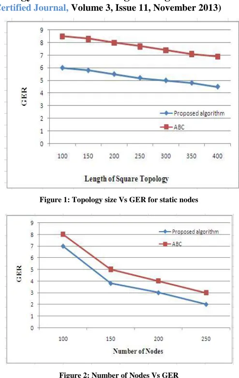
Figure 1 shows the graph between GER and the number of nodes for different Size of topology. In the proposed system simulation, it is assumed that the square fields of lengths 100m to 400m with a step of 100 and the number of nodes varied from 100 to 250 with step of 50.

[image:4.612.321.568.117.507.2]

Figure 2 shows the graph between GER and Size of topology for the different communication range of nodes. GER remains nearly constant. This shows that GER is independent of size of topology in a wireless sensor network.

[image:4.612.61.221.294.368.2]

Figure 1: Topology size Vs GER for static nodes

Figure 2: Number of Nodes Vs GER

The proposed system also has used the same metric as used in (Doherty L et al. 2001) for localization error estimation.

(5)

International Journal of Emerging Technology and Advanced Engineering

[image:5.612.48.290.228.631.2]

152

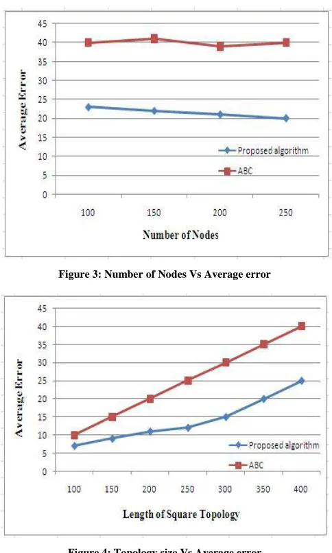
Where n is the number of sensor nodes, li denotes the actual position of the ith node and ei denotes the position estimation of the ith sensor where i = 1... n. The proposed system has used the same parameters as in GER calculations. Average localization error for different number of nodes in proposed algorithm is shown in Figure.3. The average localization error decreases with the number of nodes.

Figure 3: Number of Nodes Vs Average error

Figure 4: Topology size Vs Average error

Figure.4 shows the graph between the Average localization error and Size of topology for the different communication range of sensor nodes. The average localization error increases with the size of the topology. As GER is independent of size of topology average localization error gives better performance for localization error.

VI. CONCLUSION

This paper proposed a localization technique for wireless sensor network using internode distance. The Proposed method is very easy and efficient in terms of average localization error. GER result shows that the localization error decreases with increases in the number of nodes. Here, it is feasible to localize the sensor nodes with the average localization error in all topologies. The proposed metric average distance is capable to achieve localization in wireless sensor networks.

REFERENCES

[1 ] P. Goud, A. Sesay, and M. Fattouche, “A spread spectrum radiolocation technique and its application to cellular radio,” Proc. IEEE., Comp. and Signal Processing, pp. 661–664, 1991.

[2 ] J. Caffery and G. Stuber Jr, “Vehicle location and tracking for IVHS in CDMA microcells,” Proc. IEEE PIMRC, pp. 1227–1231, 1994. [3 ] C. Knapp and G. Carter, “The generalized correlation method for

estimation of time delay,” IEEE Trans. vol. no. 8, pp. 320–27, 1976. [4 ] G. Carter, “Time delay estimation for passive sonar signal

processing,”IEEE Trans., vol. no. 6,pp. 463–470, 1981.

[5 ] T. He et al., “SPEED: A stateless protocol for real-time communication in sensor networks,” in the Proc of International Conference on Distributed Computing Systems, May 2003. [6 ] W. Hahn and S. Tretter, “Optimum processing for delay-vector

estimation in passive signal arrays,” IEEE Trans. Inform. Theory, vol.,no. 9, pp. 608–614, 1973.

[7 ] J. Smith and J. Abel, “Closed-form least-squares source location estimation from range-difference measurements,” IEEE Trans., vol. ASSP-35, no. 12, pp. 1661–69, 1987.

[8 ] Capkun S., Hamdi M., and Hubaux J. P., “GPS free positioning in mobile Adhoc networks”, Proceedings of the 34th Hawaii International Conference on System Sciences, Maui, HI, USA; pp. 3481-3490, Jan. 2001.

[9 ] Savarese C., Rabaey J. M. and Beutel J. “Locationing in distributed ad-hoc wireless sensor networks”, Proceedings of IEEE International Conference on Acoustics, Speech, and Signal Processing, Vol.4, pp. 2037-2040, 2001.

[10 ]Priyantha N. B., Balakrishnan H., Demaine E. and Teller S. “Anchor-free distributed localization in sensor networks”, Technical Report 892, MIT Lab. for Computer Science, Apr. 2003.

[11 ]Moses R. L., Krishnamurthy D. and Patterson R.M. “A Self-Localization Method for Wireless Sensor Networks”, EURASIP Journal on Applied Signal Processing, Vol.4, pp. 348–358, 2002. [12 ]Niculescu D. and Nath B. “Ad Hoc Positioning System Using

AOA”, Proc of 22nd Annual Joint Conference of the IEEE Computer and Communications, INFOCOM, Vol.3, pp. 1734-1743, 2003.

[13 ]Fang L., Du W. and Ning P. “A beacon-less location discovery scheme for wire-less sensor networks”, Proc of 24th Annual Conference of the IEEE Computer and Communications Societies, Vol.1, pp. 161-171, 2005.

[14 ]Bulusu N., Heidemann J. and Estrin D., “GPS-less low-cost outdoor localization for very small devices”, Journal of Personal Communications, Vol.7 Iss.5, pp. 28-34, Oct. 2000.