Design of Model Predictive Control for Non Linear Process

(1)

International Journal of Emerging Technology and Advanced Engineering

Website: www.ijetae.com (ISSN 2250-2459, ISO 9001:2008 Certified Journal, Volume 6, Issue 1, January 2016)

304

Design of Model Predictive Control for Non Linear Process

B. V. Anarase

1

, B. J. Parvat

2

, C. B. Kadu

3

1_{Instrumentation & Control Engg. Dept. & Pravara Rural Engineering College, Loni (M. S.) 413736} 2,3_{Associate Professor, Instrumentation & Control Engg. Dept. & Pravara Rural Engineering College, Loni, 413736}

Abstract—This paper presents design of Model predictive

control for laboratory experiment closed loop water level system. Model predictive control uses a mathematical model to simulate a process. This model then fits the inputs to predict the system behavior. The main aim of this paper to build the Model predictive control (MPC) strategy, analyze and compare the control effects with Proportional-Integral-Derivative (PID) control strategy in maintaining a water level system. An advanced control method, MPC has been widely used and well received in a wide variety of applications in process industry, it utilizes an explicit process model to predict the future response of a process and solve an optimal control problem with a finite horizon at each sampling instant.

In this paper, we first designed and built up a closed-loop water level system. Next, we modeled the system by using experimental data of the system using system identification toolbox on MATLAB 7.5. Then, we implemented the model in a simulation environment on MATLAB 7.5. We tried both MPC and PID control methods to design the controller for the water level system, and compared the results in terms of peak time, settling time, overshoot, and steady-state error under various operational conditions including time delays. The results showed the advantage of MPC for dealing with the system dynamic over PID and could be designed for more complex and fast system dynamics even in presence of constraints.

Keywords— Model Predictive Control (MPC), FOPDT

(First Order Plus Delay Time), Proportional Integral Derivative (PID).SOPDT (Second Order Plus Delay time

).

I. INTRODUCTION

Due to the fast development of process industry, the requirements of higher product quality, better product function, and quicker adjustments to the market change have become much stronger, which lead to a demand of a very successful controller design strategy, both in theory and practice . As a closed loop optimal control method based on the explicit use of a process model, model predictive control has proven to be a very effective controller design strategy over the last twenty five years and has been widely used in Process industry such as oil refining, chemical engineering and metallurgy. [5]

The purpose of this work is to study the theory of model predictive control method, analyze and indentify the characteristics and the performance of model predictive controller compared with PID controller when being implemented in the water level control system.

PID controller is relatively simple in structure which can be easily implemented in practice. Therefore, it is widely used in process control industry. In this report, simple methods proposed by Ziegler-Nichols, Astrom Hagglund are implemented for the real time measurement of laboratory Level control system. System model for laboratory level control system using system identification toolbox of MATLAB 7.5 version is determined and this level loop is configured with SCADA. Controller performance is determined on the basis of time domain specification. The purpose of this work is also present model based PID controller for level control system which may be extended for other SISO system like flow, pressure, temperature of liquid as well as for multivariable systems. Existing control loop uses PID controller more than 90%. Since 1940’s many methods are proposed to tune PID controller but every method have some limitations. As a result, the design of PID controller still remains a challenge before researchers and engineers. For designing and tuning of a controller one should go through following steps:

 Obtain the dynamic model of a system to control.

 Specify the desired closed loop performance on the basis of known physical constraints.

 Adopt controller strategies that would achieve the desired performance.

 Implement the resulting controller using suitable platform.

 Validate the controller performance and modify accordingly if required.

1.1 PROBLEM STATEMENT

i) Determination of system model

(2)

International Journal of Emerging Technology and Advanced Engineering

305

ii)Design of Proportional Integral Derivative controller

The work elaborates a method of designing PI / PID controller with conventional Ziegler-Nichols, and Astrom Hagglund which is model based control strategy, for performance evaluation and real time implementation to level control system. The method is based on FOPDT model The objective of this work is to compute PID tuning parameters to get the better performance.

iii) Design of Model Predictive Controller

The MPC is designed for the model of level control system and is simulated in MATLAB.

Finally a comparative study is made on the performance of the PID and MPC controller getting better system parameter like Maximum overshoot , Rise time ,

Peak time Settling time , Steady state error .The

designed controller is implemented using Supervisory Control and Data Acquisition System (SCADA) and also documents a level control simulation which is performed using PID controller. All simulations were performed using MATLAB package Version 7.5 and Model Predictive Control Toolbox 2 3, Simulink toolbox (ver. 7.0) on personal computer

II. PROCESS DISCRIPTION

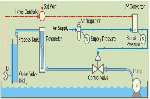
Level control trainer is designed for understanding the basic principles of level control. The process setup consists of supply water tank fitted with pump for water circulation. The level transmitter used for level sensing is fitted on transparent process tank. The process parameter (level) is controlled by microprocessor based digital indicating controller which manipulates pneumatic control valve through I/P converter. A pneumatic control valve adjusts the water flow in to the tank. These units along with necessary piping are fitted on support housing designed for table top mounting.

The controller can be connected to computer through USB port for monitoring the process in SCADA mode.

The specifications of the system are:

1.Type of Control: SCADA

2.Control Unit: Digital indicating controller with RS485 communication

3.Communication: USB port using RS 485-USB converter

4.Level Transmitter: Type Electronic ,two wire , Range 0-250 mm,Output 4-20 mA

5.I/P Convertor: Input 4-20 mA ., Output 3-15 psig 6.Control Valve :Type: Pneumatic ,Size:1/4”, Input :

3-15 psig, Air to close, Linear

7. Rota meter: 10-100 LPH

8. Process Tank: Transparent, Acrylic, with 0-100 % graduated scale

9. Air filter Regulator :Range 0-2.5 Kg/cm2

10. Pressure Range : Range 0-2.5 Kg/cm2 Range 0-7 Kg/cm2

11. Overall dimensions: 550W X 480D X 525 H mm Fig. 1 explores the system schematic arrangement of Level Control System.

Figure 1 System schematic arrangement of level control System

The example level-control problem had three critical pieces of instrumentation: a sensor (measurement device), actuator (manipulated input device), and controller. The sensor measured the tank level, the actuator changed the flow rate, and the controller determined how much to vary the actuator, based on the sensor signal. There are many common sensors used for chemical processes. These include temperature, level, pressure, flow, composition, and pH. The most common manipulated input is the valve actuator signal (usually pneumatic). Each device in a control loop must supply or receive a signal from another device. When these signals are continuous, such as electrical current or voltage, we use the term analog. If the signals are communicated at discrete intervals of time, we use the term digital.

2.1 Determination of system model

Models play a very important role in control-system design. Models can be used to simulate expected process behavior with a proposed control system..

[image:2.612.325.566.247.407.2]

(3)

International Journal of Emerging Technology and Advanced Engineering

306 The specific variables required as input data and generated as output predictions are important features of the model. The equations often stem from a numerical solution to one or more differential equations and their boundary conditions.

Thus, by definition, models require a combination of mathematics and experimental data. To be relevant, they also need to be validated with realistic measurements and finally implemented into practice.

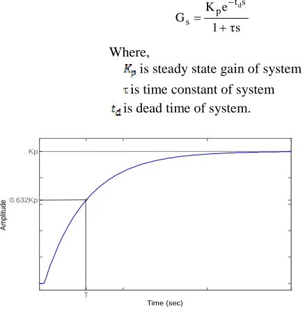
In the design of model based controller, system model is an important element. White box model requires complete and correct physical data of the system under consideration. But this data is not available for the system described. Hence, system model is determined through system identification. We used time domain step test data from the system for determination of model. We considered FOPDT model [3] This step response locates the system parameters like steady state gain, time delay and the time constant of the process from which model obtained is of general form as,

τs 1

e K G

s t p s

d

 



(1)

Where,

is steady state gain of system

is time constant of system is dead time of system.

Time (sec)

Amp

lit

u

d

e

T 0.632Kp

[image:3.612.335.548.146.344.2]

Kp

Figure 2 A typical step response of FOPDT system

Figure 3 shows a typical step response of SOPTD system. This step response locates the system parameters like peak overshoot, settling time, dead time of the system from which the model can be obtained as,

2

2 2

( )

2

d t s n

n n

e G s

s s











  (2)

Where,



n is natural frequency of system



is damping ration of system

t

d is dead time of system.

Time (sec)

A

m

pl

itu

de

td tp ts

1+Mp

Figure 3 A typical step response of SOPDT system

The system parameters

n

 and



are calculated from peak overshoot

p

M and settling time (2% criterion) tsby

solving (3) and (4) given by,

2 1

P

M

e

  



(3)

4

s n

t



 (4)

In the given system, from the open loop response of the Level Control System, it is seen that by measuring input – output data we can create the mathematical models of dynamic systems from measured input-output data by using system Identification Toolbox in MATLAB.

[image:3.612.55.274.376.602.2]

The following estimate of the plant is obtained by using system Identification Toolbox:

[image:3.612.331.555.559.707.2]

(4)

International Journal of Emerging Technology and Advanced Engineering

307 Hence, For the best fit of 90.92% shown above in figure 4 we get FOPDT model as,

) 43 . 26 1 ( 22 . 0 ) (

69 . 1

s e s

G

s p   _



(5)

III. CONTROL THEORY

3.1 Problem Definition

In the process industries, for the proper functioning of level control system we use to control the pneumatic control valve. For level control PID controller is a popular conventional approach. This scheme works satisfactorily in the absence of any process disturbances. However, when there are significant process disturbances, the PID control scheme does not perform well because of lack of knowledge of proper controller gains to cope with such disturbances. Inevitably over time and use, PID controllers get detuned. Hence, there is good motivation to investigate alternatives to this control scheme using model predictive control.

3.2 Proposed Solution

The performance of the existing PID control scheme is observed, and collected data is used to gain knowledge about the process. Based on this process knowledge, an intelligent control technique Model predictive control (MPC) is developed. The technique proposed in this was tested on a Model predictive control Toolbox. It shows that an intelligent control scheme such as MPC gives better performance in rejecting process disturbances when compared PID control scheme.

3.3 Proportional-Integral-Derivative (PID) Control

Proportional, Integral and Derivative terms are the three basic parameters of PID controller; these three terms fulfill the different requirements in the control process.

The implementation of proportional term is to make the reaction to the current error occurred in time, let the control effect take place as fast as possible and drive the error to the direction of minimization. Change this term will affect the steady state error and the dynamic performance.

The implementation of integral term is to eliminate the steady state error and accelerates the movement of the process reaching the reference value. Change this term will affect the steady state error and system stability.

The implementation of derivative term is to improve the system stability and the speed of dynamic reaction; it can also predict the future change of the error, so that an adjusted signal can be brought into the system before the error goes too large.

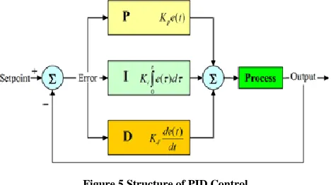
3.3.1 PID Control structure

The basic idea of PID control is to compare the system output with the set points, and minimize the error by tuning the three process control inputs.

[image:4.612.327.561.207.338.2]

The structure of PID controller is showed in Figure 5

Figure 5 Structure of PID Control

A proportional–integral–derivative controller (PID controller) is a controller which is popularly used in industrial control systems. It is fed with the error signal, that is, the difference between the reference, or the desired output and the actual output (which is obtained as a feedback). The controller then attempts to bring the actual output to track the reference.

The PID controller algorithm involves three separate constant parameters ( P, I and D respectively) and is thus, also called three- term control. P depends on the present error, I on the accumulation of past errors, and D is a prediction of future errors, based on current rate of change. The weighted sum of these three actions is given as input to the process through a control element. By tuning the three parameters, the controller provides the required control action.

If C(t) represents the controller output, which is the manipulated variable (MV(t)), that is, the process input, then:

(6)

As we can see from figure 5, in order to make the output value reach the reference value, the error between the two values is minimized by PID controller through adjusting the control input.

(5)

International Journal of Emerging Technology and Advanced Engineering

308 The implementation of proportional term is to make the reaction to the current error occurred in time, let the control effect take place as fast as possible and drive the error to the direction of minimization. Change this term will affect the steady state error and the dynamic performance. The implementation of integral term is to eliminate the steady state error and accelerates the movement of the process reaching the reference value. Change this term will affect the steady state error and system stability. The implementation of derivative term is to improve the system stability and the speed of dynamic reaction; it can also predict the future change parameter individually.

Table 1

Effects caused by increasing the PID control parameter individually

PID Control Parameter

s

Rise Time

Overshoo t

Settling time

Steady State Error

Stabilit y

p

K Decreas

e Increase

Small Change

Decreas

e Reduce

i

K Decreas

e Increase Increase

Large Decreas

e

Reduce

d

K

Small Decreas

e

Decrease Decreas e

Small Change

Therefore, tuning PID control parameters is a complicated process that we have to find an optimal way to arrange the values of the parameters for the control response. In this thesis, we used Ziegler-Nichols oscillation method, which is introduced in [1] and Astrom Hauggland method, which is introduced in [2].

3.3.2 Tuning Method of PID Control

The PID controller tuning methods are classified into two main categories – Closed loop methods, Open loop methods. Closed loop tuning techniques refer to methods that tune the controller during automatic state in which the plant is operating in closed loop . The open loop technique refer to method that tune the controller when it is in manual state and the plant operates in open loop

3.3.3 Ziegler-Nichols PID Tuning method

This pioneer method, also known as the close-loop or on-line tuning method was pro-posed by Ziegler and Nichols in 1942. Like all the other tuning methods, it consists of two steps.

1.Determination of the dynamic characteristics, or personality, of the control loop.

2.Estimation of the controller tuning parameters that produce a desired response for the dynamic characteristic determined in the ﬁrst step, in other words, matching the personality of the controller to that of the other elements in the loop.

In this method the dynamic characteristic of the process are represented by the ultimate gain of a proportional controller and the ultimate period of oscillation of the loop. It usually determinate the ultimate gain and period from the actual process by the following procedure: Switch oﬀ the integral and derivative modes of the feedback controller so as to have a proportional controller.

[image:5.612.341.543.340.443.2]

From a time recording of the controlled variable such as the ﬁgure below, the period of oscillation is measured and recorded as T the ultimate period.

Figure 6 The period of oscillation is measured and recorded as T the ultimate period

For the desired response of the close loop, Z-N method speciﬁed a decay ratio of one-fourth. The decay ratio is the ratio of the amplitudes of two successive oscilla-tions. It should be independent of the input to the system and should depend only on the roots of the characteristic equation for the loop [9]. The tuning relationship are intended to minimize the integral of the error, their use is referred to as minimum error integral tuning. However the integral of the error cannot be minimized directly, because a very large negative error would be the minimum

The strategy of the method is that first set K_iand K_dto zero while K_d as a small gain, and then gradually increase

the value of Kpuntil the value Kuthat caused the

(6)

International Journal of Emerging Technology and Advanced Engineering

[image:6.612.51.287.462.558.2]

309

Table .2

Ziegler-Nichols PID Tuning method

Type Control

Parameters

P Controlle

r

PI Controlle

r

PID Controlle

r

p

K 0.5K_u 0.45K_u 0.6K_u

i

K

u

t 2 . 1

u

t 5 . 0

1

d

K 0.125t_u

3.3.4 Astrom-Hagglund PID tuning method

Astrom and Hagglund (1985) recognized that the Ziegler-Nichols continuous cycling method actually identiﬁes the point (-l/Ku, 0) on the Nyquist curve, and moves it to a predeﬁned point. With PID-control, it is possible to move a given point on the Nyquist curve to an arbitrary position,. By increasing the gain, the arbitrary point A moves in the direction of G(jw). Changing the I or D-action moves the point in the orthogonal direction. Frequency domain characteristics, conversely, are very straightforward to obtain by means of a relay experiment. This oscillation has the frequency ox where P(j) intersects the critical point locus of the relay, which is a straight line parallel to the real negative axis, located in the third quadrant of the complex plane and depending on the hysteresis entity. Noise and disturbances are omitted here for simplicity [2].

Type Control

Parameters

PID Controller

p

K

d

Kmt T 94 . 0

i

K 2t_d

d

K 0.5t_d

The controller is a PID controller in the form of

equation (8). The system model G(s) is assumed to be known or determined experimentally. For First Order plus Time Delay (FOPTD) systems are of the form given in equation (1).

The transfer function of PID controller is:

s K s K K s T T K s

G _d _p i _d

i c

c    )  

1 1 ( )

( (7)

Where,

K_pis the proportional gain ,T_iis the integral time

T_d is the derivative time

3.3.5 Astrom Hagglund Robust Testing

Hagglund and Astrom (2002) have derived PI controller tuning rules for integrator with time-delay" processes and time-constant with time-delay" processes giving maximum performance given a requirement on robustness.[3]

Assuming the process model is in equation (1) the PI controller settings according to Hagglund and Astrom are as follows:

(8)

(9)

3.4 Model Predictive Control

The general design objective of model predictive control is to optimize, based on the computed trajectory of future manipulated variableu, predict the future behavior of the plant outputy. The optimization is performed within a limited time window by giving plant information at the start of the time window. Model Predictive Control, or MPC, is an advanced method of process controls that has been in use in the process industries such as chemical plants and oil refineries since the 1980s [9]. Model predictive controllers rely on dynamic models of the process, most often linear empirical models obtained by system identification. The applied models are determined to depict the behavior of complex dynamical systems. Hence the models are used to predict the behavior of dependent variables (i.e. outputs) of the modeled dynamical system with respect to changes in the process independent variables (i.e. inputs). In chemical processes, independent variables are most often set points of regulatory controllers that govern valve movement (e.g. valve positioners with or without flow, temperature or pressure controller cascades), while dependent variables are most often constraints in the process (e.g. product purity, equipment safe operating limits). The model predictive controller uses the models and current plant measurements to calculate future moves in the independent variables that will result in operation that honors’ all independent and dependent variable constraints. The MPC then sends this set of independent variable moves to the corresponding regulatory controller set points to be implemented in the process [14].

3.4.1 Model Predictive Control strategy

(7)

International Journal of Emerging Technology and Advanced Engineering

[image:7.612.55.283.233.386.2]

310 At each control interval an MPC algorithm attempts to optimize future plant behavior by computing a sequence of future manipulated variable adjustments. The first input in the optimal sequence is then sent into the plant, and the entire calculation is repeated at subsequent control intervals. The following is a figure 7 shows the basic idea of predictive control based on a single-input, single output plant.

Figure 7 Model Predictive Control Strategy

MPC is based on iterative, finite-horizon optimization of a plant model. At time the current plant state is sampled and a cost minimizing control strategy is computed (via a numerical minimization algorithm) for a relatively short time horizon in the future:. Specifically, an online or on-the-fly calculation is used to explore state trajectories that emanate from the current state and find a cost-minimizing control strategy until time. Only the first step of the control strategy is implemented, then the plant state is sampled again and the calculations are repeated starting from the new current state, yielding a new control and new predicted state path. The prediction horizon keeps being shifted forward and for this reason MPC is also called receding horizon control. Although this approach is not optimal, in practice it has given very good results.

3.4.2 Objective Functions Optimization Problem

The term optimization implies a best value for some type of performance criterion. This performance criterion is Known as an objective function. Here, we first discuss possible objective functions, then possible process models that can be used for MPC.

Objective Functions

Here, there are several different choices for objectives functions. The first one that comes to mind is a standard least-squares or “quadratic objective function.”

The objective function is a “sum of squares” of the predicted errors (differences between the set points and model-predicted outputs) and the control moves

A quadratic objective function for a prediction horizon of 3 and a control horizon of 2 can be written

(10)

Where ŷ represents the model predicted output ,r is the set point, ΔU is the change in manipulated input from one sample to the next ,w is a weight for the changes in the manipulated input, and the subscripts indicate the sample time (k is the current sample time ). For a prediction horizon of P and a control horizon of M,the least Squares objective function is written

(11)

Another possible objective function is to simply take a sum of the absolute values of the predicted errors and control moves.

For a prediction horizon of 3 and a control horizon of 2, the absolute value objective function is

Which has the following general form for a prediction horizon of P and a control horizon of M:

(13)

The optimization problem solved stated as a minimization of the objective function, obtained by adjusting the M control moves, subject to modeling equations (equality constraints), and constraints on the inputs and outputs.

3.4.3 Model Predictive Control structure

(8)

International Journal of Emerging Technology and Advanced Engineering

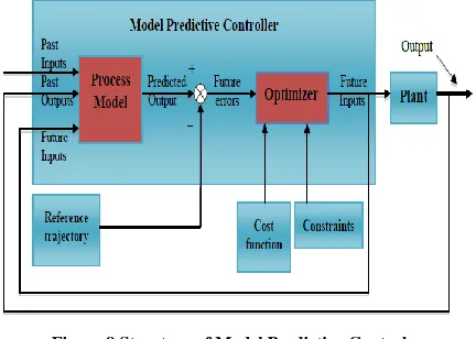
[image:8.612.64.280.236.390.2]

311 Besides, the control effort and the future errors between predicted output and reference trajectory are taken into account in the optimizer with cost function and constraints in order to get optimized future inputs which are to be sent to the plant. Then the real output of the plant will be sent back to the process model as a current value to start the next prediction horizon. The following figure 8 shows the structure of Model Predictive Control.[5]

Figure 8 Structure of Model Predictive Control

3.4.4 Model Predictive Control elements

MPC algorithm includes a dynamic model of system process; the cost function and the history of old control signals to generate the optimal control moves. From figure 8. we can see that the essence of MPC is to optimize the future behavior of the whole system process. And the very future behavior is predicted through the process model that we choose, therefore, the process model is the element to capture the dynamic process and is the most significant element of an MPC controller.

The Model Predictive Control is a model based control strategy that uses the process model to calculate the control efforts, in order to minimize an objective function without violating input or output constraints. The methodology of a predictive controller consists in predicting, at each timet,

the future outputs for a determined horizon N_p.This

prediction of the outputs is based on the model of the process and depends on the known values of past inputs and outputs up to instant t. The set of future control signals is calculated by optimizing a given criterion (called objective function or performance index) in order to keep the process as close as possible to the reference trajectory, which can be the set point or an approximation of it. The control effort is included in the objective function in most cases. Weights are used to adjust the influence of each term in the equation.

The solution to the problem is the future control sequence that minimizes the objective function equation. The constraint MPC problem is to minimize a cost function,

   

 

.

1

0

2

1

2



 

       

 p Nu

i S

N

i Q

i t u i

t r i t y

J (14)

Subject to linear inequality constraints on the system outputs, inputs and states. Here, r is the set-point; N_p

and N_u are the prediction and control horizons

respectively. Weights Qand S is used to adjust the influence of the error and inputs respectively. Once the control sequence has been obtained only the first control move is implemented. Subsequently the horizon is shifted and the values of all sequences are updated and the optimization problem is solved once again. The controller tuning parameters of the MPC are sampling time, controlled variable horizon, Prediction horizon and Weight matrices that are used in optimization procedure.

The first step of the control strategy is implemented, then the plant state is sampled again and the calculations are repeated starting from the current state, yielding a new control and new predicted state path. The prediction horizon is continuously shifted forward and for this reason MPC is also called receding horizon control. In order to get the optimal control variable, we must solve the equations (14). This is a standard quadratic programming (QP) problem of the form [7]:

. 2

1 T T

f HU U

J  (15)

Subject to

. 0

 b AU

. 0

 k LU

Here, H is a symmetric N_uN_umatrix and Aand L is u

c N

m  in size, where m_c is the total number of inequality constraints. Active set method and Interior Point method are two popular methods used to solve QP problems. In this thesis we have implemented Active Set Method for finding optimal solution of (14-15)

IV. SIMULATION RESULTS AND DISCUSSION

(9)

International Journal of Emerging Technology and Advanced Engineering

312 The measurement of the reaction time (time interval between the instant when the change occurs and when the control system will generate a corresponding command signal), the settling time (the time required for the response curve to reach and stay within a range of 2% of the final value), and the other quality indicators are performed. Moreover, an investigation on the difference between the two control algorithms is shown.

4.1 Simulation with PID controllers (Step Input)

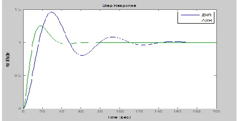
The simulation results for PID controller tuning by Ziegler-Nichols & Astrom Hagglund methods for FOPDT model (5) obtained for Level control system shown in fig. 9

Figure 9 Unit step response of Zigler Nichols & Astrom -Hagglund PID Controller for Level control system model (5)

4.2 Simulation with MPC controllers (Step Input)

[image:9.612.330.559.134.308.2]

The step response of the proposed MPC controller with the control horizon M=2, prediction horizon, P =10 without manipulated variable constraint and output variable constraint is shown in Fig.10

Figure 10 Unit step response of Model Predictive Controller for Level control system model (5)

[image:9.612.50.286.299.460.2]

Table 3 shows the performance comparison results of Model Predictive control method with the conventional PID Controllers methods on the basis of time domain specifications for Level control system (5).

Table 3

Comparison of controller performance on the basis of time domain specifications

Controllers Parameters

PID Controller

(Z-N)

PID Controller

(A- H )

MPC Controller

Peak Time ( ) sec. 30.51 14.97 0

Settling Time ( ) sec. 208.4 52.96 10 Maximum

Overshoot( ) 1.428 1.252 0

Steady State Error( ) 0 0 0

[image:9.612.325.566.400.528.2]

(10)

International Journal of Emerging Technology and Advanced Engineering

313 After simulation we have find that these entire controller have different value of parameters such as peak time(tp),

settling time(t_s), maximum overshoot(Mp), and steady

state error(e_ss). In the analysis we have seen that more accurate result came using Astrom Hagglund PID Controller over Ziegler-Nichols PID controller, further better result got in case of MPC Controller. Table 3 show that MPC controller gives better time domain specifications than PID Controller.

4.3 Robustness analysis

In order to investigate the robustness of model in presence of uncertainties, the model parameters are randomly altered. For model obtained in (5),

k

=-0.22,

d

t =1.69 sec and t_p= 26.43 sec. Let, these parameters are

deviated as much as 20% from their nominal values due to model uncertainty. Let, there is 20% increase in dead time and gain and 20% decrease in time constant.

Therefore, new model is:[7]

) 716 . 31 1 ( 264 . 0 ) (

028 . 2

s e s

G

s p   _



(16)

4.3.1 Simulation with PID controllers (Step Input)

[image:10.612.324.562.133.323.2]

The simulation results for PID controller tuning by Ziegler-Nichols & Astrom Hagglund methods for robustness analysis of FOPDT model (16) obtained for Level control system is shown in figure 11

Figure 11 Unit step response of Zigler Nichols & Astrom -Hagglund PID Controller for robustness analysis of Level control system model

(16)

4.3.2 Simulation with MPC controllers (Step Input)

The step response of the proposed MPC controller with the control horizon M=2, prediction horizon, P =10 without manipulated variable constraint and output variable constraint for robustness analysis of FOPDT model (16) is shown in Fig.12

Figure 12 Unit step response of Model Predictive Controller for Robustness analysis of Level control system model (16)

Table 4 shows the performance comparison results of Model Predictive control method with the conventional PID Controllers methods on the basis of time domain specifications for robustness analysis of Level control system (16).

Controllers Parameters

PID Controller

(Z-N )

PID Controller

(A- H)

MPC Controller

Peak Time ( ) sec. 29.9 17.8 0

Settling Time ( ) sec. 205 62.7 14 Maximum

Overshoot( ) 1.46 1.25 0

Steady State Error( ) 0 0 0

Table 4 shows the result of response of controller for robust analysis we have taken for analysis, using simulation process. These controllers have different responses for the input taken as Step. After simulation we have find that these entire controller have different value of parameters such as peak time(tp), settling time(ts), maximum

overshoot(Mp), and steady state error(ess). In the analysis

[image:10.612.328.562.416.520.2] [image:10.612.47.289.476.599.2]

(11)

International Journal of Emerging Technology and Advanced Engineering

314 V. CONCLUSION

A high performance Model based Predictive Control algorithm is proposed for the level Control process. The MPC control algorithm is compared with conventional PID control in terms of time domain specifications like settling time, overshoot, Peak time, steady state error. The Model Predictive Controller gives better performance than PID Controller for the level control system. MPC controller can adjust the control action before a change in the output set point actually occurs. Hence from the results we conclude that MPC is better than PID controller

REFERENCES

[1] J.G. Ziegler and Nichols, “Optimal Settings for Automatic Controllers”, Trans. ASME, vol. 64 P.P. 759-768, 1942.

[2] K.J. Astrom and T. Haughland, “Automatic Tuning of PID Controllers”, 1st ed. Research Triangle Park NC: Instrum.Soc. Amer, 1995.

[3] Finn Haugen, “Comparing PI tuning methods in a Real benchmarktemperature control System”, Modelling, Identification and control,Vol.31, No. 3, 2010, pp. 7991, ISSN1890- 1328 [4] K. Ogata, “Modern Control Engineering”, 3rd ed. Upper saddle

River, NJ: Prentice- Hall 1997.

[5] Ang Li M. S. 2010,Comparison between model predictive control and pid control for water-level maintenance in a two-tank system. University of Pittsburgh.

[6] J.Prakash and K.Srinivasan, “Design of nonlinear PID controller and nonlinear model predictive controller for a continuous stirred tank reactor”, ISA transactions, Vol.48, issue 3, July 2009, page no. 273 – 282.

[7] R.A. Darandale, C. B.Kadu and C.Y.Patil ,”Design of Model Predictive Control for Temperature Process” , Proc. of Int. Conf. on Advances in Signal Processing and Communication

[8] Alberto Bemporad, N., Lawrence Ricker, James Gareth Owen, “Model Predictive Control - New tools for design and evaluation.” Proceeding of the 2004 American Control Conference Boston, Massachusetts June 30. July 2, 2004.

[9] S. Joe Qin, Thomas A. Badgwell, “A survey of industrial model predictive control technology”, Control Engineering Practive 11, 733-764, 2003.

[10] http://en.wikipedia.org/wiki/Model_predictive_control

[11] J.M. Maciejowski, “Predictive Control with Constraints”, Prentice Hall, Harlow, 2001.

[12] http://en.eikipedia.org/wiki/PID_controller

[13] B. Wayne Bequette, “Process Control Modeling, Design and Simulation”, Prentice Hall (2003), ISBN: 0-13-353640-8.

[14] M. Morari and N. L. Ricker, Model Predictive Control Toolbox, The Mathworks, Inc., Natick, MA, 1994