Analytic Solution of MHD Stagnation Point Flow over a Stretching Permeable Surface with Effects of Viscous Dissipation and Joule Heating

http://dx.doi.org/10.4236/eng.2014.612077

Analytic Solution of MHD Stagnation Point

Flow over a Stretching Permeable Surface

with Effects of Viscous Dissipation and Joule

Heating

Satyaban Panigrahi, Motahar Reza

Department of Mathematics, National Institute of Science and Technology, Berhampur, India Email: [email protected], [email protected]

Received 11 September 2014; revised 26 October 2014; accepted 11 November 2014

Copyright © 2014 by authors and Scientific Research Publishing Inc.

This work is licensed under the Creative Commons Attribution International License (CC BY). http://creativecommons.org/licenses/by/4.0/

Abstract

A mathematical analysis is investigated to obtain an analytic solution of magneto hydrodynamic stagnation-point flow towards permeable stretching surface with viscous dissipation and joule heating. In the presence of uniform suction, a transverse magnetic field normal to the surface is applied when the surface is stretched in its own plane with a velocity proportional to the distance from the stagnation-point. The governing nonlinear momentum and energy equations are solved by homotopy analysis method (HAM) to obtain the complete analytic solution and a good agree-ment is found. The convergence region shows the validity of the HAM solutions. It is observed that the velocity at a point increases/decreases more with increase in the magnetic parameter when the free stream velocity is greater/less than the stretching velocity in presence of suction. An teresting result of the analysis is that, in the presence of suction parameter, the temperature in-creases with the increase in magnetic parameter at a certain distance from the stretching surface. Near stagnation point on the surface, heat flows from the surface to the fluid and far from the stagnation-point, heat flows from the fluid to surface due to combining effect of ohmic dissipation and strain energy inside the boundary layer.

Keywords

MHD, Suction, Stretching Surface, Homotopy Analysis Method

1. Introduction

applica-tions in several technologies of process industry. A number of manufacturing industries process and include both metal and polymer sheets during the production of sheeting materials. This kind of motion of a fluid close to the rigid or stretching surface can be investigated from a standard boundary layer equation. The quality of the final product depends to a large extent on the rate of heat transfer at the stretching surface. It is, therefore, of in-terest to know the fluid behavior over a stretching surface which determines the rate of cooling. Hiemenz [1]

first analyzed an exact solution of the stagnation point flow of a viscous fluid over a rigid surface. The axisym-metric three-dimensional cases for the rigid surface are investigated by Homann [2]. The steady flow of an in-compressible viscous fluid over an elastic sheet was studied by Crane [3] where the flow being caused solely by stretching of sheet in its own plane. The temperature distribution in the flow over a stretching surface subject to uniform heat flux was studied by Dutta et al. [4]. The steady two-dimensional orthogonal stagnation point flow of an incompressible viscous fluid towards a stretching surface which is held at constant temperature, was inves-tigated by Mohapatra and Gupta [5]. Later, Mohapatra and Gupta [6] extended his work to study the momentum and heat transfer characteristic of stagnation-point flow of a viscoelastic fluid over a stretching surface. Hassa-nien [7] analyzed the similarity solution for the flow and heat transfer of a viscoelastic fluid over a stretching sheet. The temperature distribution for the stagnation point flow of a micro polar fluid past a stretching sheet was investigated by Nazar et al. [8].

In the region of adverse pressure gradient the flow in a boundary layer separates. Due to separation, it leads to increase in drag on the body immersed in the flow and adversely affects heat transfer from the surface of the body. Flow separation can be prevented by applying suction to remove the directed fluid particle from the boundary layer. On the other hand, the wall shear stress and hence friction drag is reduced by blowing. Wall suction and blowing have many applications such as turbine blade cooling, transition delay and prevention se-paration. The effect of suction on the Hiemenz problem was studied by Schlichting and Bussmann [9]. An ap-proximate solution to the problem of uniform suction is given by Ariel [10]. The effect of uniform suction on the Homann problem where the flat plate oscillates in its own plane is considered by Weidman and Mahalingam

[11]. The effect of uniform suction or injection on the two- or three-dimensional stagnation-point flow of a con-ducting fluid was given by Attia [12] [13] in the presence of an externally applied uniform magnetic field. The effect of uniform suction or injection on two-dimensional stagnation point flow towards a stretching surface with heat generation was given by Attia and Seddeek [14].

Electrically conducting fluid like a liquid metal, electrolyte or plasma under the influence of magnetic field induces electric current. This type of fluid has many applications in industries, for example, to drive flow, in-duce stirring, levitation or control heat transfer and turbulence. An exact similarity solution to the MHD boun-dary layer equations for the steady two-dimensional flow of an electrically conducting incompressible fluid due to the stretching of a plane elastic surface in the presence of a uniform transverse magnetic field was given by Pavlov [15]. Chakrabarti and Gupta [16] studied the MHD flow of a Newtonian fluid over a stretching sheet. In the presence of uniform transverse magnetic field Andersson [17] investigated the MHD flow of a viscoelastic fluid past a stretching surface. Liao [18] developed Homotopy analysis method (HAM) which is one of the most successful and efficient methods to solve a non-linear differential equation. This method is based on a funda-mental concept in topology, i.e., Homotopy (Hilton [19]) which is widely used in numerical techniques (Grigo-lyuk and Shalashilin [20]).

In this present work, HAM is employed to find the new analytic solution of the effect of uniform transverse magnetic field as well as suction or blowing on a steady two-dimensional orthogonal stagnation point flow of an electrically conducting fluid towards a permeable stretching surface. For a very small magnetic Reynolds num-ber the induced magnetic field can be neglected. We assume the wall and free stream temperature to be constant.

2. Flow Analysis

Consider the two dimensional stagnation point flow of a viscous incompressible electrically conducting fluid impinging orthogonally to a permeable stretching surface coinciding with plane y=0, the being in the region

0

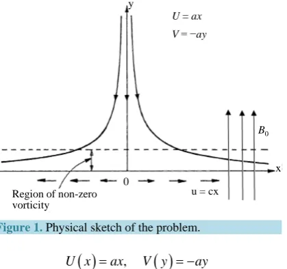
y> . Two equal and opposite forces are applied to the sheet along the x-axis such that the surface is stretched keeping the origin fixed as shown inFigure 1. The flow is permeated by a uniform magnetic field of strength

0

B applied transverse to the plate. The plate is assumed to be electrically non-conducting and is subject to uni-form suction or blowing.

[image:3.595.212.422.86.283.2]

Figure 1. Physical sketch of the problem.

( )

,

( )

U x =ax V y = −ay (1)

where a>0 is proportional to the free stream velocity far away from the surface. Under these assumptions, along with the Boussinesq approximation and boundary layer approximations, the governing equations for the steady two-dimensional stagnation point flows by introducing Lorentz force are

0

u v

x y

∂ ∂

+ =

∂ ∂ (2)

( )

(

)

2 2 0 2 B

u u U u

u v U U x u

x y x y

σ ν

ρ

∂ ∂ ∂ ∂

+ = + + −

∂ ∂ ∂ ∂ (3)

(

)

2 2 2 2 0 2 P P

T T T u

u v B u ax

x y y c y c

µ σ κ ρ ρ   ∂ ₊ ∂ ₌ ∂ ₊ ∂ _{+ −}  

∂ ∂ ∂ _∂ _ (4)

where T represents the temperature and ρ , µ, ν, σ ,

κ

and cP are the density, the viscosity, the

ki-nematic viscosity, these electric conductivity of the fluid, thermal diffusivity and the specific heat of the fluid at constant pressure, respectively, and U x

( )

is horizontal component of the inviscid potential flow velocity over the body surface. At the stretching surface, the velocity in the x direction is equal to the moving surface ve-locity cx, where c is a positive constant. So boundary conditions are

0

at

, , W 0

u=cx v= −v T =T y= ₍₅₎

( )

, as

u→U x T →T∞ y→ ∞ (6)

where v0 is the constant velocity at the plate with v0>0 for suction and v0<0 for blowing and TW and

T∞ are constants with TW >T∞.

To examine the flow regime, we introduce the following similarity transformation

( )

( )

( )

( )

,

, , , ,

W

T x y T c

u cxf v c f x y

T T

η ν η θ η η

ν ∞ ∞ − ′ = = − = =

− (7)

Here prime denotes differentiation with respect to η. Using above equation, the continuity Equation (2) is satisfied automatically and Equations (3) and (4) becomes

2

2 2

2 0

a a

f ff f H f

c c

 

′′′+ ′′− ′ + _ − ′_+ =

  (8)

( )

(

)

(

)

2 2 2

2

2 2 0

2

2

P W P W

a

B cx f

c x f c

xf f

x c T T c T T

σ

θ θ κ θ

η ν η _∞ ρ _∞

 _{′ −} 

 

′′

∂ ∂ ∂ _{ }

′ − = + +

∂ ∂ ∂ − − (9)

u = cx Region of non-zero

vorticity

x B0

0

where H B0

c

σ ρ

= is the Hartman Number. Setting

( )

, 0

( )

2 1

( )

cx x

θ η θ η θ η

ν

= + (10)

In Equation (9) and equating the coefficients of x0 and x2 we obtain the following equations for θ η0

( )

and θ η1

( )

:

0 Prf 0 0

θ′′+ θ′= (11)

(

)

( )

2 2 2

1 Pr 1 2 1 Pr. . Pr. .

a

f f E f E H f

c θ′′+ θ′− ′θ = − ′′ − _ ′− _

  (12)

where E=νc cP

(

TW−T∞

)

, is the Eckert number which is a measure of viscous dissipation.

The corresponding boundary conditions (5) and (6) can be written as

( )

0 ,

( )

0 1 ,

( )

a

f A f f

c

′ ′

= = ∞ = (13)

( )

( )

0 0 1, 0 0

θ = θ ∞ = (14)

( )

( )

1 0 0, 1 0

θ = θ ∞ = (15)

Here v0

A cν

= ± is the suction parameter (A>0 for suction and A<0 for injection). For boundary layer

flow, the wall skin friction τw is given by

0 w y u y τ µ =  ∂  =  _∂ 

  (16)

Using U x

( )

=ax as a characterized velocity, the skin friction coefficient Cf can be defined as

2 w f C U τ ρ

= (17)

Substituting (7) and (16) in (17) we get

( )

0

f x

C Re = f′′ (18)

where Rex =xU ν is the local Reynolds number.

3. Homotopy Analysis Solution

The velocity f

( )

η and the temperature θ η0

( )

, θ η1

( )

can be represented in terms of a set of base function

exp 1 : 0, 0 are integers

m a

n m n

c

η η

 _{− −}  _{≥ ≥} 

   

 

  (19)

as

( )

, 0 0 exp 1 m n m n m a

f a n

c

η ∞ ∞ η η

= =

 

= _− − _

 

∑ ∑

(20)

( )

0 , 0 0 exp 1 m n m n m a b n c

θ η ∞ ∞ η η

= =

 

= _− − _

 

∑ ∑

(21)

and

( )

1 , 0 0 exp 1 m n m n m a c n c

θ η ∞ ∞ η η

= =

 

= _− − _

 

where an m, , bn m, and cn m, are the coefficients. Looking into the boundary condition and the base function we

choose the initial guess f0

( )

η , θ0,0

( )

η and θ η1,0

( )

as

( )

0 1 exp 1 sgn 1

a a a

f A

c c c

η = + η− −_ _− − η__ _ − _

 

 

  (23)

( )

0,0 exp 1

a c θ η = _− − η_

  (24)

and

( )

1,0 exp 1 1 exp 1

a a

c c

θ η = _− − η__ − _− − η_

    (25)

The auxiliary linear operators L_f , 0

L_θ and 1

L_θ can be taken as

( )

3

( )

3 2

( )

2

d ; d ;

; 1

d d

f

f q a f q

L f q

c η η η η η = + −  

  (26)

( )

( )

( )

( )

0 1

2

2

d ; d ;

; ; 1

d d

q a q

L q L q

c

θ θ

θ η θ η

θ η θ η

η η

= = + −

   

    (27)

where q∈

[ ]

0,1 is an embedding parameter. The auxiliary linear operators L_f , 0

L_θ and 1

L_θ satisfies

1 2 3exp 1 0

f

a

L C C C

c η η    + + − − =     

  (28)

0 4 5exp 1 0

a

L C C

c

θ η

 ₊ _{− −} ₌

  

 

  (29)

1 6 7exp 1 0

a

L C C

c θ η    + − − =     

  (30)

where Ci,

(

i= −1 7

)

are arbitrary constants.

Corresponding to the governing differential Equations (8), (11) and (12), we define the non-linear operators as

( )

( )

( )

( )

( )

2

3 2 2

2 2

3 2 2

ˆ _; ˆ _; ˆ _; ˆ _;

ˆ _; ˆ

f

f q f q f q f q a a

N f q f H H

c c

η η η η

η η η η η   ∂ ∂ ∂ ∂ _{ }   = + −  − + _{ }+

  _{∂ ∂} _{ ∂} _{ ∂  } (31)

(

) (

)

(

)

(

)

0

2

2

ˆ _; ˆ _;

1

ˆ ˆ

ˆ _{; , ;}

Pr

q q

N_θ θ η q f η q θ η f θ η

η η

∂ ∂

  = +

  _{∂ ∂} (32)

( ) ( )

( )

( )

( )

( )

( )

1 2 2 2 2 2 2 2

ˆ ˆ ˆ

ˆ _; ˆ _{; ; ; ;}

1

ˆ ˆ

ˆ _{; , ; 2}ˆ

Pr

q q f q f q f q a

N q f q f E EH

c

θ

θ η θ η η η η

θ η η θ

η η η

η η

   

∂ ∂ ∂ ∂ ∂

  = + − +   +  − 

  ∂ ∂ ∂ _ ∂ _ _ ∂ _ (33)

If hf , hθ0, hθ1 denotes the non-zero auxiliary parameters and Gf

( )

η , Gθ0

( )

η , Gθ1

( )

η denotes the

auxiliary function, we construct the zero-th order deformation equations

(

1−q L

)

f fˆ

(

η;q

)

− f0

( )

η =h Gf f

( )

η Nffˆ

(

η;q

)

 (34)

(

)

0 0

(

)

0

( )

0 0

( )

0 0

(

)

ˆ ˆ

1−q Lθ _θ η;q −θ η _=h Gθ θ η Nθ _θ η;q _ (35)

(

)

1 1

(

)

1

( )

1 1

( )

1 1

(

)

ˆ ˆ

subject to the boundary conditions,

( )

( )

( )

0

ˆ _; ˆ _;

ˆ _{0; ,} f q _1, f q a

f q A

c η η η η η η = →∞ ∂ ∂ = ∂ = =

∂ (37)

( )

( )

( )

( )

0 1 0 1

ˆ _{0;q 1,} ˆ _{0;q 0,} ˆ _{;q 0,} ˆ _{;q 0}

η η

θ θ θ η θ η

→∞ →∞

= = = = (38)

where

( )

0

( )

1

( )

exp 1

f

a

G G G

c

θ θ

η = η = η = _− − η_

  (39)

When q=0 and q=1 we have

( )

0,

( )

( )

ˆ _{; 0} ˆ _;1

f η = f f η = f η (40)

( )

( )

( )

0 0,0, 0

ˆ _{; 0} ˆ _;1

θ η =θ θ η =θ η (41)

( )

( )

( )

1 1,0, 1

ˆ _{; 0} ˆ _;1

θ η =θ θ η =θ η (42)

Note that when the embedding parameter q increases from 0 to 1, fˆ

(

η;q

)

, θ ηˆ₀

(

;q

)

and θ ηˆ₁

(

;q

)

varies

from the initial approximations f0

( )

η , θ0,0

( )

η and θ η1,0

( )

to the exact solution f

( )

η , θ η0

( )

and

( )

1

θ η respectively. By Taylor’s theorem we express fˆ

(

η;q

)

, θ ηˆ0

(

;q

)

and θ ηˆ1

(

;q

)

in the power series of the embedding parameter q.

( )

0

( )

( )

1

ˆ _; m

m m

f η q f η f η q

∞

=

= +

∑

(43)

( )

( )

( )

0 0,0 0,

1

ˆ _{; 0} m

m m

q

θ η θ η ∞ θ η

=

= +

∑

(44)

( )

( )

( )

1 1,0 1,

1

ˆ _{; 0} m

m m

q

θ η θ η ∞ θ η

=

= +

∑

(45)

where

( )

(

)

0 ; 1 ! m m m q f q f m η η η ₌ ∂ =

∂ (46)

( )

0

(

)

0, 0 ; 1 ! m m m q q m θ η θ η η ₌ ∂ =

∂ (47)

( )

1

(

)

1, 0 ; 1 ! m m m q q m θ η θ η η ₌ ∂ =

∂ (48)

If the auxiliary parameters hf , hθ0 and hθ1 are properly chosen such that the series converges at q=1

then we have

( )

0

( )

( )

1 m m

f η f η f η

∞

=

= +

∑

, (49)

( )

( )

( )

0 0,0 0,

1 m m

θ η θ η ∞ θ η

=

= +

∑

, (50)

( )

( )

( )

1 1,0 1,

1 m m

θ η θ η ∞ θ η

=

Differentiating the zero-th-order Equations (34), (35), (36) m-times with respect to the embedding parameter

q, then setting q=0, and finally dividing by m!, we have m-th-order deformation equation

( )

1

( )

( ) ( )

f

f m m m f f m

L _f η −χ f ₋ η _=h G η R η (52)

( )

( )

( )

0

( )

0 0,m m 0,m 1 0 0 m

Lθ θ η −χ θ − η =h Gθ θ η Rθ η (53)

( )

( )

( ) ( )

1

1 1,m m 1,m1 1 1 m

L_{θ }θ η −χ θ ₋ η _=h G_{θ θ} η Rθ η (54)

subject to the boundary conditions

( )

0 0,

( )

0 0,

( )

0

m m m

f = f′ = f′ ∞ = (55)

( )

( )

0,m 0 0, 0,m 0

θ = θ ∞ = (56)

( )

( )

1,m 0 0, 1,m 0

θ = θ ∞ = (57)

where

( )

1

(

)

2

2 2

1 1 1 1 2

0

1

m f

m m n m n n m n m m

n

f a a

R f f f f f H H

c c

η − − − − − − − χ

=

 

′′′ ′′ ′ ′

= + − − ′ + − _ + _

 

∑

, (58)

( )

0

1

0, 1 0, 1

0 1

Pr

m

m m n m n

n

Rθ η θ fθ

−

− − −

=

′′ ′′

= +

∑

, (59)

( )

(

)

1

2 1

2 2 2

1, 1 1 2 1, 1 1, 1 1 1

0

1

2 1 2

Pr

m

m m m m n m n n m n n m n n m n

n

a a

R EH f EH f f Ef f EH f f

c c

θ _{η θ χ} − _{θ θ}

− − − − − − − − − −

=

′′ ′ ′ ′ ′ ′′ ′ ′

= − + − +

∑

− + + (60)

and

0 1

1 , , 1

m

m

m χ _{= } ≤

>

 (61)

Let fm

( )

η ∗

, θ0,m

( )

η ∗

, θ1,m

( )

η ∗

denote the special solution of Equations (52), (53) and (54). We have

( )

( )

1

( ) ( )

1

f

m m m f f f m

f∗ η =χ f ₋ η +h L− _G η R η _, (62)

( )

( )

( )

0

( )

0 0 0

1

0,m m 0,m 1 h L G Rm

θ

θ θ θ

θ∗ η χ θ η − η η

−  

= + _{ }, (63)

( )

( )

( ) ( )

1

1 1 1

1

1,m m 1,m1 h L G Rm

θ

θ θ θ

θ∗ η χ θ η − η η

−  

= + _{ }. (64)

where 1 f L− ,

0 1

L_θ− , 1 1

L_θ− denotes the inverse operator of L_f, , L_θ0 L_θ1 respectively. Thus the solution of the m-th-

order deformation equations as

( )

( )

1 2 3exp 1

m m

a

f f C C C

c η ₌ ∗ η _{+ +} η₊ _{− −} η

 

  (65)

( )

( )

0,m 0,m 4 5exp 1

a

C C

c θ η ₌θ∗ η _{+ +} _{− −} η

 

  (66)

( )

*

( )

1,m 1,m 6 7exp 1

a

C C

c θ η =θ η + + _− − η_

  (67)

Here the integral constants Ci,

(

i=1, 2, 3,, 7

)

are determined by the boundary conditions (55), (56) and

(57) as

( )

0,

( )

1 3 2 3

0

, , 1

0 0

1

m

m

f

C C f C C

( )

( )

4 0, 5 0,m 0 , 6 0, 7 1,m 0

C = C = −θ∗ C = C = −θ∗ (69)

Therefore, it is easy to solve linear non-homogeneous Equations (52), (53) and (54) subject to the boundary conditions (55), (56) and (57) by using MATHEMATICA one after other in the order m=1, 2, 3,

4. Convergence of Homotopy Solutions

We observed that the Equations (52), (53) and (54) consist of the auxiliary parameters hf , hθ0 and hθ1. These

auxiliary parameters are important in controlling the convergence of series solutions the functions f

( )

η ,

( )

0

θ η and θ η₁

( )

. For this analysis, the admissible values of h_f , 0

h_θ and 1

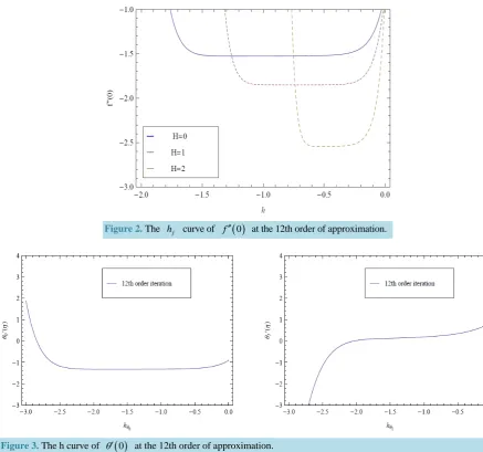
h_θ curves are plotted for 12th-

order of approximations.Figure 2 shows the admissible values of hf of f′′

( )

0 for 12th-order of

approxima-tion with a c=0.1 for several values of H. It is observed that hf curves have parallel lines segment that

correspond to the regions −1.5≤h_f ≤ −0.3, −1.0≤h_f ≤ −0.2 and −0.6≤h_f ≤ −0.3 for H=0,1, 2,

respec-tively. To analyze the admissible range of h_θ0 and h_θ1 of θ0′

( )

0 and θ1′

( )

0 are displayed in Figure 3 for

12th-order of approximation with a c=0.1, H=2 and Pr=5.0. It is observed that the converging ranges

are −2.3≤h_θ0 ≤ −0.5 and −1.8≤h_θ1≤ −0.7. From these figures we have examined that by choosing the

val-ues of convergence control parameter from these range we will get the convergent result up to higher decimal place.

5. Results and Discussion

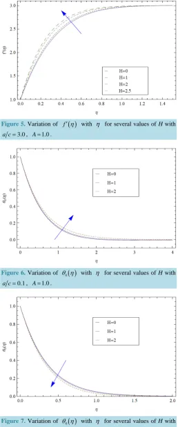
The nonlinear boundary value problem given by Equations (8), (11) and (12) with boundary conditions (13), (14), and (15) cannot be solved in closed form. So these equations are solved by Homotopy Analysis Method (HAM) to get an analytical solution. Extensive calculation has been performed by using symbolic computation software MATHEMATICA to obtain the velocity and temperature profiles for various values of physical para-meter such as Suction parapara-meter A, Hartmann Number H, Prandtl number Pr, Eckert number E, (which charac-terizes viscous dissipation in the flow) and the parameter a c (ratio of external velocity and stretching veloci-ty). Figure 4 shows the variation of horizontal velocity component with distance from the surface for several values of Hartmann Number H in the presence of suction parameter A=1.0 and a c=0.1 i.e., stretching velocity more than the straining velocity. It can be viewed that horizontal velocity decreases with increase in Hartmann Number H. It is interesting that the flow has inverted boundary layer structure because of stretching velocity cx exceeds the velocity of external stream ax (i.e. a c<1). Whereas, in the presence of suction parameter A=1.0 and a c=3, the velocity increases with increase in H, as shown inFigure 5.

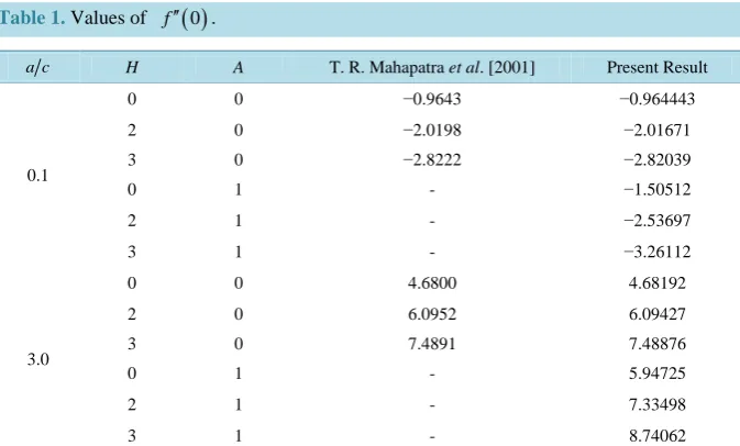
Table 1shows the value of dimensionless wall shear stress i.e., skin-friction coefficient (see Equation (18)) for several values of H and a c in the presence of suction. It gives that for fixed value of suction parameter

1

A= , the magnitude of the wall shear stress increases with increase in H and a c. In order to have correctness of our analytical result, we have examined the comparison result in the value of −f′′

( )

0 for different values of

A and H in the present study and with the corresponding values by Mahapatra et al. [21] (shown inTable 1). It is observed that during the motion of electrically conduction fluid, a certain amount of energy is stored up in the fluid as strain energy and some energy is lost due to viscous and ohmic dissipation. So in the fluid flow, energy is balanced by the internal energy, the conduction of heat, the convection of heat with the flow, the gen-eration of heat with the flow, the gengen-eration of heat through viscous and ohmic dissipation, the strain (or defor-mation) energy in the fluid and energy due to wall suction effect. At a distance X (Dimensionless length) from stagnation-point, the temperature distribution consists of two functions, first part of temperature distribu-tion denoted by θ η0

( )

which depends on the Hartmann Number and suction parameter and second part de-noted by θ η1

( )

which depends on viscous dissipation and Joule Heating.

In the presence of suction parameter A=1.0, the variation of temperature distribution θ η0

( )

with η is displayed inFigure 6 for several values of Hartman Number H with Pr=5.0, a c=0.1. It is observed that for fixed value of Pr, A=1.0, the temperature at point increases with increase in the Hartman Number when

0.1

[image:9.595.88.526.81.490.2] [image:9.595.167.541.293.720.2]

Figure 2.The h_f curve of f′′

( )

0 at the 12th order of approximation.

Figure 3.The h curve of θ′

( )

0 at the 12th order of approximation.

Figure 4.Variation of f′

( )

η with η for several values of H with

0.1

[image:10.595.184.443.85.705.2]

Figure 5. Variation of f′

( )

η with η for several values of H with

3.0

a c= , A=1.0.

Figure 6.Variation of θ η0

( )

with η for several values of H with

0.1

a c= , A=1.0.

Figure 7. Variation of θ η₀

( )

with η for several values of H with

3.0

[image:10.595.187.442.96.381.2]

[image:11.595.145.482.84.287.2]

Table 1. Values of f′′

( )

0 .

a c H A T. R. Mahapatra et al. [2001] Present Result

0.1

0 0 −0.9643 −0.964443

2 0 −2.0198 −2.01671

3 0 −2.8222 −2.82039

0 1 - −1.50512

2 1 - −2.53697

3 1 - −3.26112

3.0

0 0 4.6800 4.68192

2 0 6.0952 6.09427

3 0 7.4891 7.48876

0 1 - 5.94725

2 1 - 7.33498

3 1 - 8.74062

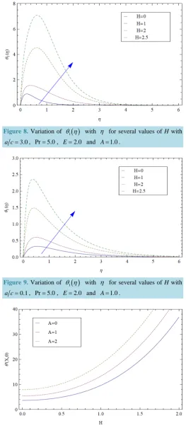
suction, viscous and ohmic dissipation and stored deformation energy in the flow

(

E=0

)

, the variation of the temperature distribution given by θ η1

( )

with η is shown inFigure 8, for several values of H with Pr=5.0 and a c>1. It is observed that a novel result, that in the presence of suction parameter A=1.0, θ η1

( )

in-creases with the increase in Hartmann Number H where as in the absence of suction parameter Mahapatra et al.

[22] shows that in the vicinity of the stretching surface θ η1

( )

increases with increase in H but after a certain distance from the stretching plate, the trend reverse.Figure 9 depicts that the variation of θ η1

( )

with η for several values of H with Pr=5.0 and A=1.0 when a c=0.1.

The dimensionless rate of heat transfer at the surface η =0 given −θ′

(

X, 0

)

from Equation (10) is derived as

(

)

0

( )

( )

2 1

, 0 0 0

X X

θ′ θ′ θ′

− = − − (70)

where

1 2

c

X x

υ

  =  

  . The dimensionless heat flux at the surface −θ′

(

X, 0

)

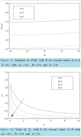
is computed from Equation (70)

and displayed inFigure 10 andFigure 11 corresponding two distinct locations

(

X =0.1

)

and

(

X =2.0

)

on the stretching surface. It is observed fromFigure 10 that the heat flows from the surface to fluid at the small value X =0.1 (for several values of H), because −θ′

(

X, 0

)

. On the side, for X =0.1, it is seen inFigure 11

that the heat flow from the fluid to the stretching surface for several value of H because −θ′

(

X, 0

)

is negative. It is more interesting that heat flux is more in the presence of suction. This novel result can be interpreted phys-ically that for small value of X =0.1, the term 2 ₁

(

)

, 0

X θ′ X

− becomes small and both ohmic dissipation and strain energy in the flow are not playing important roles to generate heat. So for small value of X, heat flows from the surface to fluid since Tw>T∞. But for the large value of X =3.0, the term 1

(

)

2

, 0

X θ′ X

− has

sig-nificant role due combine effect of ohmic dissipation and strain energy inside the boundary layer which causes to generate sufficient heat inside the boundary layer. Thus, the temperature of the fluid near the surface exceeds the surface temperature Tw. So heat flows from fluid to surface even when Tw>T∞. In this case it is also ob-served that heat flux increase with suction for fixed value of H.

[image:11.595.144.482.87.291.2]

[image:12.595.181.445.83.690.2]

Figure 8. Variation of θ η₁

( )

with η for several values of H with

3.0

a c= , Pr=5.0, E=2.0 and A=1.0.

Figure 9. Variation of θ η₁

( )

with η for several values of H with

0.1

a c= , Pr=5.0, E=2.0 and A=1.0.

Figure 10. Variation of θ′

( )

0 with H for several values of A at 2.0

[image:13.595.184.443.78.517.2]

Figure 11. Variation of θ′

( )

0 with H for several values of A at 0.1

X = with a c=0.1, Pr=5.0 and E=2.0.

Figure 12. Value of X₀ with E for several values of H with 0.1

a c= , Pr=5.0 and A=1.0.

6. Conclusion

The present study describes the effect of viscous dissipation and joule heating on magneto hydrodynamic stag-nation-point flow towards permeable stretching surface. To analyze the new analytic solution of this problem, we apply homotopy analysis method. By this powerful and newly developed technique, the convergence series solutions are obtained. To validate the analytic solutions of velocity distribution and temperature distribution using HAM method, we have computed the convergence regions. The HAM solutions have an excellent agree-ment. A novel result of this problem is that the temperature increases with the increase in Hartmann Number H

at a certain distance from the stretching surface in the presence of suction parameter. Heat flows from the sur-face to the fluid at near stagnation point on the sursur-face and on the hand far from the stagnation-point, heat flows from the fluid to surface due to combining effect of ohmic dissipation and strain energy inside the boundary layer.

References

[2] Homann, F. (1943) Der einfluss grosser zahighkeit bei der stromung um den zylinder und um die kugel. Zeitschrift für Angewandte Mathematik und Mechanik, 16, 153-164. http://dx.doi.org/10.1002/zamm.19360160304

[3] Crane, L.J. (1970) Flow Past a Stretching Plate. Zeitschrift für Angewandte Mathematik und Physik, 21, 645-647.

http://dx.doi.org/10.1007/BF01587695

[4] Dutta, B.K., Roy, P. and Gupta, A.S. (1985) Temperature Field in Flow over a Stretching Surface with Uniform Heat Flux. Int. Comm. International Communications in Heat and Mass Transfer, 12, 89-94.

http://dx.doi.org/10.1016/0735-1933(85)90010-7

[5] Mahapatra, T.R. and Gupta, A.S. (2002) Heat Transfer in Stagnation-Point Flow towards a Stretching Sheet. Heat and Mass Transfer, 38, 517-521. http://dx.doi.org/10.1007/s002310100215

[6] Mahapatra, T.R. and Gupta, A.S. (2004) Stagnation Point Flow of a Viscoelastic Fluid. The International Journal of Non-Linear Mechanics, 39, 811-820. http://dx.doi.org/10.1016/S0020-7462(03)00044-1

[7] Hassanien, I.A. (2002) Similarity Solutions for Flow and Heat Transfer of a Viscoelastic Fluid over a Stretching Sheet Extruded in a Cross Cooling Stream. Zeitschrift für Angewandte Mathematik und Mechanik, 82, 409-419.

http://dx.doi.org/10.1002/1521-4001(200206)82:6<409::AID-ZAMM409>3.0.CO;2-1

[8] Nazar, R., Amin, N., Filip, D. and Pop, I. (2004) Stagnation Point Flow of a Micropolar Fluid towards a Stretching Sheet. International Journal of Non-Linear Mechanics, 39, 1227-1235.

http://dx.doi.org/10.1016/j.ijnonlinmec.2003.08.007

[9] Schlichting, H. and Bussmann, K. (1943) Exakte Losungen fur die Laminare Grenzchicht mitAbsaugung und Ausbla-sen. Schriften der Deutschen Akademie der Luftfahrtforschung B, 7, 25-69.

[10] Ariel, P.D. (1994) Stagnation Point Flow with Suction: An Approximate Solution. Journal of Applied Mechanics, 61, 976-978. http://dx.doi.org/10.1115/1.2901589

[11] Weidman, P.D. and Mahalingam, S. (1997) Axisymmetric Stagnation Point Flow Impinging on a Transversely Oscil-lating Plate with Suction. Journal of Engineering Mathematics, 31, 305-318.

http://dx.doi.org/10.1023/A:1004211515780

[12] Attia, H.A. (2003) Hydromagnetic Stagnation Point Flow with Heat Transfer over a Permeable Surface. Arabian Journal for Science and Engineering, 28, 107-112.

[13] Attia, H.A. (2003) Homann Magnetic Flow and Heat Transfer with Uniform Suction or Injection. Canadian Journal of Physics, 81, 1223-1230. http://dx.doi.org/10.1139/p03-061

[14] Attia, H.A. and Seddeek, M.A. (2007) On the Effectiveness of Uniform Suction or Injection on Two Dimensional Stagnation-Point Flow towards a Stretching Surface with Heat Generation. Chemical Engineering Communications,

194, 553-564. http://dx.doi.org/10.1080/00986440600992537

[15] Pavlov, K.B. (1974) Magneto Hydrodynamic Flow of an Incompressible Viscous Fluid Caused by the Deformation of a Plane Surface. Magnitnaya Gidrodinamika, 4, 146-147.

[16] Chakrabarti, A. and Gupta, A.S. (1979) Hydromagnetic Flow and Heat Transfer over a Stretching Sheet. Quarterly of Applied Mathematics, 37, 73-78.

[17] Andersson, H.I. (1992) MHD Flow of a Viscoelastic Fluid Past a Stretching Surface. Acta Mechanica, 95, 227-230.

http://dx.doi.org/10.1007/BF01170814

[18] Liao, S.J. (1992) The Proposed Homotopy Analysis Technique for the Solution of Nonlinear Problems. Ph.D. Thesis, Shanghai Jiao Tong University, Shanghai.

[19] Hilton, P.J. (1953) An Introduction to Homotopy Theory. Cambridge University Press, Cambridge.

[20] Grigolyuk, E.E. and Shalashilin, V.I. (1991) Problems of Nonlinear Deformation: The Continuation Method Applied to Nonlinear Problems in Solid Mechanics. Kluwer Academic Publishers, Kluwer.

http://dx.doi.org/10.1007/978-94-011-3776-8

[21] Mahapatra, T.R. and Gupta, A.S. (2001) Magnetohydrodynamic Stagnation-Point Flow towards a Stretching Sheet.

Acta Mechanica, 152, 191-196. http://dx.doi.org/10.1007/BF01176953

[22] Mahapatra, T.R., Dholey, S. and Gupta, A.S. (2007) Momentum and Heat Transfer in Magneto Hydrodynamic Stagna-tion-Point Flow of a Viscoelastic Fluid towards a Stretching Surface. Meccanica, 42, 263-272.