Complexity Reduced MIMO Interleaved SC FDMA Receiver with Iterative Detection

(1)

http://dx.doi.org/10.4236/ijcns.2014.712051

Complexity Reduced MIMO Interleaved

SC-FDMA Receiver with Iterative Detection

Masaki Tsukamoto, Yasunori Iwanami

Department of Computer Science and Engineering, Graduate School of Engineering, Nagoya Institute of Technology, Nagoya, Japan

Email: [email protected], [email protected]

Received 11 October 2014; revised 21 November 2014; accepted 1 December 2014

This work is licensed under the Creative Commons Attribution International License (CC BY).

http://creativecommons.org/licenses/by/4.0/

Abstract

In this paper, we propose the receiver structure for Multiple Input Multiple Output (MIMO) Inter-leaved Single Carrier-Frequency Division Multiple Access (SC-FDMA) where the Frequency Do-main Equalization (FDE) is firstly done for obtaining the tentative decision results and secondly using them the Inter-Symbol Interference (ISI) is cancelled by ISI canceller and then the Maximum Likelihood Detection (MLD) is used for separating the spatially multiplexed signals. Furthermore the output from MLD is fed back to ISI canceller repeatedly. In order to reduce the complexity, we replace the MLD by QR Decomposition with M-Algorithm (QRD-M) or Sphere Decoding (SD). Moreover, we add the soft output function to SD using Repeated Tree Search (RTS) algorithm to generate soft replica for ISI cancellation. We also refer to the Single Tree Search (STS) algorithm to further reduce the complexity of RTS. By examining the BER characteristics and the complexity reduction through computer simulations, we have verified the effectiveness of proposed receiver structure.

Keywords

Interleaved SC-FDMA, MLD, QRD-M, Sphere Decoding, RTS, STS, Iterative Detection, Complexity Reduction

1. Introduction

(2)

be-comes a problem [1]-[3]. The SC-FDMA is used as the uplink wireless scheme in LTE (Long Term Evolution). The feature of its low Peak to Average Power Ratio (PAPR) characteristics decreases the burden of amplifier li-nearity in User Equipment (UE) and the SC-DFMA is more suitable to uplink transmission than Orthogonal Frequency Division Multiplexing (OFDM) [4]. Moreover by employing the interleaved SC-FDMA where the subcarriers for each UE are deployed like a comb tooth, the PAPR of SC-FDMA is further reduced and the fre-quency diversity effect becomes large. We have already proposed the MIMO SC-FDE and MIMO Interleaved SC-FDMA receivers with iterative detection where the receive signal is firstly detected by FDE, i.e., MMSE nulling, to obtain the tentative decision results and secondly the ISI cancellation from the receive signal using the tentative decision results is done followed by the MLD for separating spatially multiplexed signals [5]. However, as the complexity of MLD increases as the power of modulation levels to the number of transmit an-tenna, the complexity reduction of MLD becomes an important issue. For reducing the complexity of MLD, QRD-M is proposed [6], but it is a quasi-Maximum Likelihood (ML) method and could not obtain the ML solu-tion although the complexity is greatly reduced. On the other hand, SD [1] [2] can obtain the ML solution like MLD with reduced complexity. In this paper, we propose the novel receiver structure in which the MLD is re-placed by QRD-M or SD to reduce the complexity of MLD [5]. In addition, by using RTS algorithm [7], we add the bit LLR output function on SD, which enables the proposed SD receiver to cancel the ISI with the soft repli-ca resulting in more accurate ISI repli-cancellation. Moreover we have replaced the RTS by the STS [8] algorithm to further reduce the complexity of RTS. Through computer simulations, we have examined the BER characteris-tics and the complexity reduction effect of proposed MIMO interleaved SC-FDMA iterative receiver with ISI canceller and MLD, QRD-M, SD with RTS or STS. Consequently we verify that the receiver structure using STS mostly improves the BER and the complexity.

2. MIMO Interleaved SC-FDMA Receiver

2.1. Proposed Transmitter and Receiver Structure

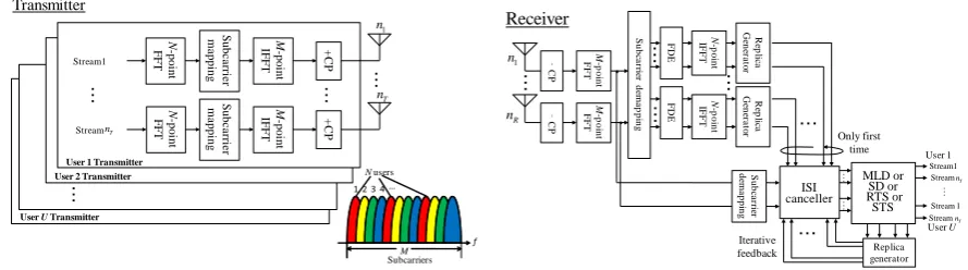
In Figure1, the block diagram of transmitter and receiver for the uplink is shown. At the transmitter of each UE, the Quadrature Amplitude Modulation (QAM) modulated signal is Fast Fourier Transform (FFT) transformed with N-points and converted to the frequency domain. The FFT points are then mapped to the interleaved fre-quency points like a comb tooth. After that, the frefre-quency points are Inverse FFT (IFFT) transformed with M

points (M =4N in case of 4 UE’s for example) to obtain the time domain signal. The Cyclic Prefix (CP) is in-serted and the signal is transmitted to the channel. At the receiver in Base Station (BS), after removing the CP, the FDE, i.e., MMSE nulling, is firstly done. The receive signal is then FFT converted with M points and the frequency domain signal is obtained. The frequency points are de-mapped to each user subcarrier arrangement and the subcarriers are multiplied by the MMSE weight Gu

( )

n at frequency point n, i.e.

( )

{

( ) ( )

}

1

2

T

H H

u n u n u n u n nTσ n

−

= +

G H H H I (1)

where Hu

( )

n denotes the MIMO channel matrix at the frequency point n assigned to the user u

(

u=1 ~U

)

, σ2

the variance of noise at each frequency point,

T

n

I the identity matrix with the size nT

which is the number of transmit antenna. After that, the frequency points are IFFT transformed with N points and the time domain signal to be detected is obtained as ˆxu.

[

1

]

û= û ,,ûk,,ûN

x x x x (2)

We call ˆxu as the tentative decision through FDE. Using ˆxu, the receive signal replica due to ISI caused by

the transmit signals other than the signal at time k to be detected, is generated and is subtracted from the re-ceive signal. Using tentative decision result of (2) and by letting the transmit signal of user u at time k being 0, the tentative decision result for ISI cancellation is obtained as (3).

( ) ( )

1,1 1 ,1 1 ,1 ,1

1,2 1 ,2 1 ,2 ,2

\ 1 1 1

1, 1 , 1 , ,

ˆ ˆ 0 ˆ ˆ

ˆ ˆ , ,ˆ , 0,ˆ , ,ˆ ,

ˆ ˆ 0 ˆ ˆ

T T T T

u u k u k uN

u k u u k u k uN

u n u k n u k n uN n

x x x x

− +

 

 

 

=_ __{= } _

 

 

 

      

 

(3)

[image:3.595.88.533.90.214.2]

Figure 1. Block diagram of MIMO SC-FDMA transmitter and the proposed receiver structure with iterative feedback.

Next, xˆu k\ in (3) is transformed to frequency domain signal of Xˆu k\ using FFT with N points. The fre-

quency domain ISI replica is made through multiplying Xˆu k\

( )

n by the channel matrix Hu

( )

n and the ISI

replica Hu

( )

n Xˆu k\

( )

n is subtracted from the receive signal in frequency domain. Accordingly, the ISI com-

ponents due to the transmit signals other than time k are removed. If the ISI cancellation is perfect, then the condition where only the transmit signals at time k from nT transmit antennas are transmitted to the receiver

is achieved. The ISI cancelled receive signal Zu k

( )

n in frequency domain is expressed as

( )

\

,11 ,12 ,1 \ ,1

1

2 ,21 ,12 ,2 \ ,2

, 1 , 2 , \ ,

ˆ ˆ ˆ , ˆ T T

R _R _R _{R T} _T

u k u u u k

u u u n u k

u

u u u u n u k

un u n u n u n n u k n

n n n n

H n H n H n X n

Y n

Y n H n H n H n X n

= −                   =_ _−_ __ _              _{ } _{ } _         

Z Y H X

(4)

where Yu

( )

n is the receive signal of user u in frequency domain. Next, for Zu k

( )

n in (4), the signal sepa-

ration of spatially multiplexed transmission is done using MLD. The total number of candidates of receive rep-lica for MLD is _KnT_{, where} _K_{is the modulation levels. The candidate signal for MLD in time domain} _ˆ

u k

x

is obtained by letting the transmit signals all 0 except for at time k to be detected.

[

]

,1

,2

,

ˆ

0 0 0 0

ˆ

0 0 0 0

ˆ 0 0 ˆ 0 0

ˆ

0 0 0 0

T

uk

u k uk

uk n x x x       = _{= } _             _ _  

x x (5)

where the matrix size is nT×N. xˆu k in (5) is then FFT transformed with N points resulting in Xˆu k

( )

n .

( )

ˆ

u k n

X is then multiplied by the channel matrix of Hu

( )

n which is assigned for user u at frequency point n

and the candidate receive replica for MLD is obtained as Hu

( )

n Xˆu k

( )

n . Then the squared distance between

the ISI cancelled receive signal and the candidate MLD replica in frequency domain is calculated as

( )

2

1

ˆ

N

u k u u k

n

n n n

=

−

∑

Z H X (6)

where ∗ denotes the Euclidian norm. (6) is minimized over the total nT

K MLD candidates and the MLD output of ˆxuk in (5) which minimizes (6) is obtained. The tentative decision result ˆxuk in (2) is then replaced

by the obtained ˆxuk and the procedure proceeds from time k to time k+1 where the initial value of k is 1.

This ISI canceller with MLD procedure is sequentially done from time 1 to N. Accordingly the residual ISI components in tentative FDE decision results are more precisely removed and the spatially multiplexed signals

N -poi nt FFT S ubc a rri e r m a ppi ng M -poi nt IFFT + CP Stream1 ・・・・・・

User 1 Transmitter User 2 Transmitter

User U Transmitter

・

StreamnT

N -poi nt FFT S ubc a rri e r m a ppi ng M -poi nt IFFT + CP ・・・ Transmitter 1 n T n M Subcarriers Nusers f

1 2 3 4 …

‐ CP M -p oi nt FFT ・・・ ‐ CP M -p oi nt FFT ・・・ F DE S u b ca rr ier de m a p pi ng N -p oi nt IFFT S u b ca rr ier de m a ppi ng R ep lica G en er a to r R ep lica G en er a to r ・・・・・・・・・・・・ Replica generator … … N -p oi nt IFFT F DE ISI canceller Receiver Only first time Iterative feedback User 1 Stream1 StreamnT

User U Stream 1 StreamnT

(4)

are more accurately separated. After the processing for one FFT block is done, the obtained decision results for one block are regarded as the evolved tentative decision results. Then the MLD outputs are fed back to the ISI canceller at each FFT block and this feedback is iteratively done to lower the final BER.

2.2. Complexity Reduction of MLD by QRD-M or SD

The number of candidate replicas in MLD increases exponentially as _KnT _{. As the complexity reduction method}

of MLD, we illustrate the method utilizing the tree search of MLD with QR decomposition [6]. The receive sig-nal vector is written as

= +

y Hx n (7) where y is the receive signal vector with nR×1, H the frequency flat channel matrix with nR×nT , x

the transmit signal vector with nT×1 and n the receive noise vector with nR×1. Using the QR

decomposi-tion, the channel matrix is decomposed into H=QR, where Q is the unitary matrix and R is the upper tri-angular matrix. By multiplying the Hermitian transpose QH by y from the left hand side, we obtain

H H

= +

 

y QRx n

Q y Rx Q n

y Rx n

(8)

where y=Q yH and n=Q nH . The MLD criterion is then expressed as

2

2 2 2

ˆ ˆ ˆ ˆ

ˆ=argmin − ˆ =argmin − ˆ =argmin H − H ˆ =argmin − ˆ

x x x x

x y Hx y QRx Q y Q QRx y Rx (9)

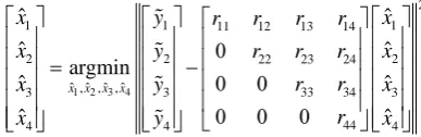
[image:4.595.224.418.410.473.2] [image:4.595.201.430.588.695.2]

As R is the upper triangular matrix, the detection of transmit signal is considered as the tree search problem from ˆxn_T where ˆxnT denotes the transmit signal candidate from antenna nT. The tree structure is shown in

Figure 2 when K=2 (BPSK) and nT =4, where the diverging number at each node and the depth of tree become K =2 and nT =4 respectively. Equation (9) is also expressed in elements as

1 2 3 4

2

1 1 11 12 13 14 1

2 2 22 23 24 2

ˆ ˆ, ,ˆ,ˆ ₃₃ ₃₄

3 3 3

44

4 4 4

ˆ ˆ

argmin

ˆ ˆ

x x x x

x y r r r r x

x y r r r x

r r

x y x

r

x y x

      

    ₀  

 ₌  ₋  

    0 0  

    ₀ ₀ ₀  

      

     

   

(10)

As the tree search method for Figure 2 toward the width direction, M algorithm is widely known. At each step, the squared distance norm for every branch is calculated, and arbitral m survival paths with the least cu-mulative squared distance metric are retained. The complexity of M algorithm is constant when the value of

m is determined and the QRD-M algorithm reduces the complexity of MLD very much, especially when

1

m= . But it could not obtain the ML solution, i.e., quasi-ML. On the other hand, the SD algorithm searches the tree of Figure 2 toward the depth direction. The SD first determines the initial sphere radius C= y−Rxˆ for some transmit candidate of xˆ. Next SD searches the transmit signal vector which falls within the radius C

toward the depth direction. When the cumulative distance metric exceeds the initial radius, then the subsequent

Figure 2. Tree structure of MLD when using QR decomposi-

tion.

Depth first search

Breadth first search

4 ˆ

x

3 ˆ

x

2 ˆ

x

1 ˆ

(5)

search along the path is no more needed, thus the amount of calculation is saved. Therefore, when the initial sphere radius is small, the complexity reduction becomes more effective. In other words, the higher the Eb N0

and the smaller the initial sphere radius is, more effectively the complexity reduction is done. If the cumulative distance metric does not exceeds the initial radius till the bottom of tree, then the initial radius is replaced by the cumulative metric and the new radius is set. In the same manner the tree search is done for every path in the tree, thus the SD can obtain the ML solution.

2.3. Receiver Structure When Using QRD-M Algorithm

By using QRD-M instead of MLD in the receiver structure in Figure 1, we reduce the complexity of MLD. The same signal processing procedure mentioned in 2 is done to cancel the residual ISI and to satisfy the condition as if only the transmit signal at time k is transmitted. After the ISI cancellation, the QRD-M is applied instead of MLD. The number of transmit signal candidates xˆ_{u k} equals _KnT _{. Like in (5), the time domain transmit signal}

vector with N points in which the candidate transmit signal is located at time k and the transmit signals at other time instants are all set to 0 is generated. Then the time domain signal vector is transformed to the fre-quency domain signal vector Xˆu k

( )

n using FFT with N points.

Then the channel matrix Hu

( )

n assigned to user u at subcarrier number n is QR decomposed.

( )

( ) ( )

u n = u n u n

H Q R (11)

The Hermitian transpose QuH

( )

n is multiplied by the output Zu k

( )

n of the ISI canceller from the left

hand side.

( )

H

( )

, 1, ,

u k n = u n u k n n= N

 _

Z Q Z (12)

The squared metric for minimization using Zu k

( )

n in (12) is given by

( )

2

,1

/ ,1 ,11 ,12 ,1

,22 ,2

/ ,2 ,2

1

,

/ , ,

ˆ ( )

ˆ 0

( )

ˆ

0 0

( )

T T

R T

R T

u k

u k u u u n

N

u u n

u k u k

n

u n n

u k n u k n

X n

Z n R n R n R n

R n R n

Z n X n

R n

Z n X n

=

 

   

 

   

 

   

−  

   

 

   

 

  _ __ _

   

∑

 _

 _

     

 

(13)

Using M algorithm, (13) is step by step calculated from the bottom to the top. The m survival paths with the least cumulative metrics are retained at each step from the bottom. The path which minimizes (13) is finally selected from the m survival paths which reach the top. The path obtained by ORD-M determines the output

ˆ_uk

x . The signal processing afterward is the same as MLD.

2.4. Receiver Structure When Using SD Algorithm

By using SD instead of MLD in the receiver structure in Figure 1, we reduce the complexity of MLD. The same signal processing procedure mentioned in 2 is done to cancel the residual ISI and to satisfy the condition as if only the transmit signal at time k is transmitted. In the proposed SD, the initial radius is set using QRD-M. (13) is used for the search of initial radius using QRD-M. The cumulative metric with small radius is firstly searched in the tree using QRD-M and we set this cumulative metric as the initial radius. Next the transmit signal candi-date which satisfies the initial radius is searched toward the depth direction in the tree. When the cumulative distance metric exceeds the initial radius, then the subsequent search along the path is no more needed, thus the amount of calculation is saved. If the cumulative distance metric does not exceeds the initial radius till the bot-tom of tree, then the initial radius is replaced by the cumulative metric and the new radius is set. In the same manner, the tree search is done for every path in the tree, thus the SD can obtain the ML solution. In (13) the search procedure is done toward the upward direction with exhaustive search to obtain the ML solution of ˆxuk.

If the QRD-M can find a smaller initial radius, then more effectively the tree search is done.

2.5. Realization of Soft Output in SD

(6)

the 2nd bit of the transmit signal from antenna i 1,

(

= ,nT

)

are given by (14) and (15) respectively.

( )

_{( )}

( )

2

( )

_{( )}

( )

2

1, , ,1 0 , ,1 1

1 1

ˆ ˆ

LLR min min 2

N N

i u k u u k i u k u u k i

n n

n n n n n n σ

= =

    

≅ −_ _ − _+ _ − __

   



∑

Z R X

∑

Z R X  (14)

( )

_{( )}

( )

2

( )

_{( )}

( )

2

2, , ,2 0 , ,2 1

1 1

ˆ ˆ

LLR min min 2

N N

i u k u u k i u k u u k i

n n

n n n n n n σ

= =

    

≅ −_ _ − _+ _ − __

   



∑

Z R X

∑

Z R X  (15)

( )

, ,1 0

ˆ

u k i n

X in (14) denotes the transmit signal in frequency domain of u-th user at time k and frequency point n from transmit antenna i with the 1st bit being 0. Xˆu k i, ,1 1_{( )}

( )

n in (14) has the same notation but with

the 1st bit being 1. Xˆu k i, ,2 0_{( )}

( )

n and Xˆu k i, ,2 1( )

( )

n in (15) represent the same notation but with the 2nd bit be-

ing 0 and 1 respectively. In SD, there exist some paths for which searches are not made in the tree. In order to calculate the bit LLR, the path for bit “0” and the path for bit “1”, both of which have minimum path metrics, have to be evaluated. For this evaluation, we have used the RTS [7] and STS [8] algorithms.

2.6. RTS Algorithm

In RTS, using (13) and the M algorithm, the path with minimum path metric is obtained firstly and is re-garded as the initial radius of SD. Then, the path metric which is not yet searched is calculated through SE algo-rithm [1] [2]. In RTS, to evaluate the bit LLR, the SE algorithm is repeatedly applied to calculate the path metric which is not searched in SD. In Figures 3(a)-(c), we show the tree structure for BPSK when the number of transmit antenna is 3, for example. In Figure 3(a), the red line shows the minimum path metric [101] obtained from the M algorithm with m=1. In this case, in order to obtain the bit LLR of xˆ3, we have to find the

minimum path metric for which xˆ3 =0, which is illustrated in Figure 3(b). Likewise, in order to obtain the bit

LLR’s of xˆ2 and xˆ1, we have to find the minimum path metrics for which xˆ2 =1 and xˆ1=0, those are

illu-strated in Figure 3(c) andFigure 3(d) respectively. To find the minimum path metrics having the counter bits, we repeatedly use the SE algorithm.

2.7. STS Algorithm

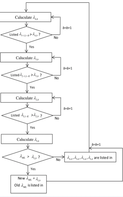
In STS, the path metrics for calculating the bit LLR’s are evaluated using the single search of the tree. The basic idea of STS follows that every path metric and its search depth are stored in the list and monitored. When the evolution of all the path metrics in the list does not occur during the tree search, the search of specific branch is saved and this results in complexity reduction. At the initial stage, the values in the list are all set to infinity. In Figure 4, we show the STS algorithm where the number of transmit antenna is 4, the number of modulation lev-el K, λs b, the accumulated norm with the search depth s and the symbol number b, λML the

accumu-lated norm of ML sequence. Also, the list as an example is illustrated in Figure 5 where the number of transmit antenna is 4 and the QPSK modulation is used.

In STS algorithm, the list inFigure 5 is filled up with the algorithm inFigure 4. When λ_3,2 is calculated for example, its value is compared with all λ1~ 2,1~ 4 already stored in the list. At this stage, when λ3.2<λ1~ 2,1~ 4, we find that the further search of this branch does not lead to the evolution of the path metric. Accordingly we stop the search and move to the calculation of λ3.3. When λML is finally obtained, the needed norms are read from

the list and the bit LLR’s are calculated using (14) and (15).

3. Computer Simulation Results

Computer simulations are made for the system in Figure 1. The simulation conditions are listed in Table 1.

(7)

(a) (b)

[image:7.595.73.537.78.320.2]

(c) (d)

Figure 3. Tree search algorithm in RTS. (a) Path with minimum path metric; (b) Paths for calculating the minimum counter path metrics for antenna 3; (c) Paths for calculating the minimum counter path metrics for antenna 2; (d) Paths for

calculating the minimum counter path metrics for antenna 1.

Figure 4. STS algorithm.

1 0 1 1 1 0 0 0 1 1 1 0 0 0

[111] [011] [101] [001] [110] [010] [100] [000] 3 ˆ x 2 ˆ x 1 ˆ x 1 0 1 1 1 0 0 0 1 1 1 0 0 0 3 ˆ x 2 ˆ x 1 ˆ x

[111] [011] [101] [001] [110] [010] [100] [000]

1 0 1 1 1 0 0 0 1 1 1 0 0 0 3 ˆ x 2 ˆ x 1 ˆ x

[111] [011] [101] [001] [110] [010] [100] [000]

1 0 1 1 1 0 0 0 1 1 1 0 0 0 3 ˆ x 2 ˆ x 1 ˆ x

[111] [011] [101] [001] [110] [010] [100] [000]

4,

Caluculate λb

4,b λ

Listedλ3~1,1~K> ?

Yes

No

b=b+1

3,

Caluculate λb

3,b λ

Listedλ2~1,1~K> ?

Yes

No

b=b+1

2,

Caluculate λb

2,b λ

Listedλ1,1~K > ?

Yes

No

b=b+1

1,

Caluculate λb

?

Yes

No ML

λ > λ1,b

1,b λ NewλML=

4,b, 3,b, 2,b, 1,b

λ λ λ λ are listed in

OldλMLis listed in

[image:7.595.204.419.363.707.2]

(8)

Figure 5. Example of list with 4 transmit antennas and the

modulation level K.

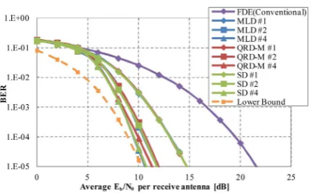
Figure 6. Comparison of BER characteristics of MIMO inter-

leaved SC-FDMA receiver with hard replica cancellation of ISI.

Table 1. Simulation condition.

Number of UE 4

Number of transmit antennas in each UE 4

Number of receive antennas at BS 4

Modulation formats QPSK

Number of total subcarriers M = 256

Number of subcarriers assigned to each user N = 64

Symbol length of QPSK T

Cyclic prefix length 4T/

Channel model between each transmit and receive antenna Equal power 16 paths quasi-static Rayleigh fading channel

Interval of delay time T/4

Subcarrier assignment IFDMA

Channel estimation Perfect at BS

FDE Nulling (MMSE)

Initial radius setting for SD (SE algorithm) QRD-M (m = 1)

Number of iterative feedbacks in the receiver 0,1,3 ( # 1)= − # denotes the

repetition number of MLD, QRD-M, SD, RTS or STS

Search depth

Symbol number

Already calculated Not calculated 1

Sym Sym2 Sym3 Sym4

4,1

λ

3,1

λ

2,1

λ

1,1

λ

4,2

λ

3,2

λ

2,2

λ

1,2

λ

∞

2,4

λ

1,4

λ

1,3

λ

2,3

λ

∞

3,3

λ

_3,4

1

S=

2

S=

3

S=

4

S=

[image:8.595.205.428.87.252.2] [image:8.595.203.426.285.423.2]

(9)

Figure 7. Comparison of BER characteristics of MIMO inter-

leaved SC-FDMA receiver with soft replica cancellation of ISI.

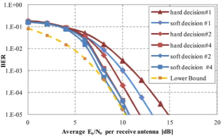
Figure 8. Comparison of BER characteristics of MIMO interleaved SC-FDMA receiver between hard decision and soft de-

cision with iterative feedback.

the lower bound of BER where the ISI cancellation is perfect, which means the demodulated bits for ISI cancel-lation are error-free. In Figure 9, we show the comparison of complexity of MLD, QRD-M, SD, RTS and STS on 4 4× flat fading channel. This complexity is measured using “tic” and “toc” function in MATLAB and the computation time needed for MLD is normalized to unity.

From Figure 6, compared with the conventional FDE receiver, the proposed receiver using MLD with no iterative feedback improves the BER by about 7 dB at BER=10−5. By increasing the number of iterative feedbacks, the proposed receiver further improves the BER and obtains the BER improvement of more than 10 dB which is close to the lower bound of BER. This is because the MLD outputs with high reliability are used as the improved decision results for making the accurate ISI replicas. Accordingly more exact ISI cancellation be-comes possible followed by improved MLD performance. We observe the BER performance of QRD-M is infe-rior to MLD, but the BER of SD coincides with the MLD, thus the SD can obtain the ML solution.

From Figure 7, we see that the BER performance with soft ISI cancellation behaves basically the same as the SD with hard ISI cancellation in Figure 6, but the BER approaches more rapidly to the lower bound than the hard ISI cancellation. We find that at average Eb N0 =8 dB

( )

the BER coincides with the lower bound and

this means the perfect ISI cancellation is possible at this receive SNR value.

FromFigure 8, we see that the soft ISI cancellation with iterative feedback performs better than the hard rep-lica cancellation. This is because more accurate ISI reprep-lica for cancellation can be generated for the soft decision than the hard decision.

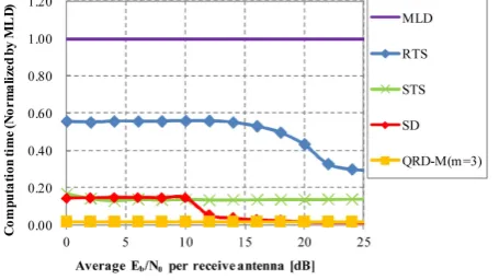
From Figure 9, QRD-M, SD, RTS and STS can reduce the computation time compared with MLD. The QRD- M is the most effective in reducing the computation time. The computation time is almost 1/100 of MLD and is constant over the average Eb N0 value. However, QRD-M is sub-optimal and ML solution is not obtained.

[image:9.595.205.423.87.223.2] [image:9.595.203.427.263.399.2]

(10)

[image:10.595.204.432.93.221.2]

Figure 9. Comparison of computation time among MLD, QRD-

M, SD, RTS and STS on flat fading channel.

time is about 15 times higher than QRD-M. However, above Eb N0=10 dB

( )

, the computation time ap-

proaches to QRD-M. This is because for high average Eb N0 region, the initial radius can be set to a very

small value. Although the RTS can produce the soft output, the RTS needs a lot of path metric calculation lead-ing relatively high computation time. The STS which is the improved version of RTS shows the computation time almost the same as the SD in low Eb N0 region. Therefore it can reduce the computation time about 1/5

compared with the RTS. However, the computation time of STS is almost constant over entire Eb N0 region.

4. Conclusion

In this paper, we have proposed the low BER receiver structure for the interleaved SC-FDMA on the uplink MIMO frequency selective fading channels. In the proposed receiver, using the tentative decision results ob-tained from the MMSE nulling (FDE), the ISI components are cancelled and the MLD is then used for separat-ing the spatially multiplexed signal streams. The reliable output from MLD is again fed back to the ISI canceller to reduce the residual ISI. Furthermore we improve the complexity of MLD by replacing it with QRD-M or SD. We have verified the BER characteristics of the proposed receiver with MLD, QRD-M or SD through computer simulations. The receiver with SD achieves the same BER as the one with MLD, i.e., ML solution, whereas the QRD-M has the inferior BER because of its quasi-ML solution. We have also verified that the complexity of SD is very much improved compared with MLD especially in high Eb N0 region. In order to cancel the ISI more

effectively using soft replica, we have further replaced the SD by RTS or STS algorithm in which the soft out from SD is available. As a result, the BER characteristic approaches more rapidly to the lower bound. The com-plexity of STS is lower than the RTS and almost coincides with the SD in low Eb N0 region. The proposed

receiver structure will be useful to extend the coverage of uplink.

Acknowledgements

This study has been supported by the Scientific Research Grant-in-aid of Japan No. 24560454 and Sharp coop-eration.

References

[1] Guo, Z. and Nilsson, P. (2004) Reduced Complexity Schnorr-Euchner Decoding Algorithms for MIMO Systems. IEEE

Communications Letters, 8, 286-288. http://ieeexplore.ieee.org/stamp/stamp.jsp?tp=&arnumber=1300579

http://dx.doi.org/10.1109/LCOMM.2004.827376

[2] Shim, B. and Kang, I. (2008) Sphere Decoding with a Probabilistic Tree Pruning. IEEE Transactions on Signal

Processing, 56, 4867-4878. http://ieeexplore.ieee.org/stamp/stamp.jsp?tp=&arnumber=4626106

http://dx.doi.org/10.1109/TSP.2008.923808

[3] Vikalo, H. and Hassibi, B. (2002) Maximum-Likelihood Sequence Detection of Multiple Antenna Systems over Dis-persive Channels via Sphere Decoding. EURASIP Journal on Applied Signal Processing, 2002, Article ID: 156743.

(11)

[4] Myung, H.G., Lim, J. and Goodman, D.J. (2006) Single Carrier FDMA for Uplink Wireless Transmission. IEEE

Vehi-cular Technology Magazine, 1, 30-38. http://ieeexplore.ieee.org/stamp/stamp.jsp?tp=&arnumber=4099344

http://dx.doi.org/10.1109/MVT.2006.307304

[5] Moriyama, M. and Iwanami, Y. (2012) Complexity Reduction Using QRD-M or SD in MIMO Interleaved SC-FDMA Receiver with Iterative Detection. International Symposium on Information Theory and Its Applications, Honolulu, 28-31 October 2012, 145-149. http://ieeexplore.ieee.org/stamp/stamp.jsp?tp=&arnumber=6400904

[6] K.J., Kim, Jiang, Y., Iltis, R.A. and Gibson, J.D. (2005) A QRD-M/Kalman Filter-Based Detection and Channel Esti-mation Algorithm for MIMO-OFDM Systems. IEEE Transactions on Wireless Communications, 4, 710-721.

http://ieeexplore.ieee.org/stamp/stamp.jsp?tp=&arnumber=1413237

http://dx.doi.org/10.1109/TWC.2004.842951

[7] Studer, C. and Burg, A. (2008) Soft-Output Sphere Decoding: Algorithms and VLSI Implementation. IEEE Journal on

Selected Areas in Communications, 26, 290-300. http://ieeexplore.ieee.org/stamp/stamp.jsp?tp=&arnumber=4444760

http://dx.doi.org/10.1109/JSAC.2008.080206

[8] Studer, C. and Bölcske, H. (2010) Soft-Input Soft-Output Single Tree-Search Sphere Decoding. IEEE Transactions on

Information Theory, 56, 4827-4842. http://ieeexplore.ieee.org/stamp/stamp.jsp?tp=&arnumber=5571884

(12)