Collecting Statistical Methods for the Analysis of Climate Data as Service for Adaptation Projects

http://dx.doi.org/10.4236/ajcc.2015.41002

Collecting Statistical Methods for the

Analysis of Climate Data as Service for

Adaptation Projects

Barbara Hennemuth1, Steffen Bender1, Katharina Bülow1, Norman Dreier2, Peter Hoffmann3_{, Elke Keup-Thiel}1_{, Christoph Mudersbach}4

1_{Climate Service Center 2.0, Helmholtz-Zentrum Geesthacht, Hamburg, Germany}

2_{Hamburg University of Technology, Institute of River and Coastal Engineering, Hamburg, Germany} 3_{German Meteorological Service, Hamburg, Germany}

4_{Bochum University of Applied Sciences, Institut für Wasser und Umwelt, Bochum, Germany}

Email: [email protected]

Received 18 December 2014; accepted 6 January 2015; published 3 March 2015

Copyright © 2015 by authors and Scientific Research Publishing Inc.

This work is licensed under the Creative Commons Attribution International License (CC BY).

http://creativecommons.org/licenses/by/4.0/

Abstract

The development of adaptation measures to climate change relies on data from climate models or impact models. In order to analyze these large data sets or an ensemble of these data sets, the use of statistical methods is required. In this paper, the methodological approach to collecting, struc-turing and publishing the methods, which have been used or developed by former or present ad-aptation initiatives, is described. The intention is to communicate achieved knowledge and thus support future users. A key component is the participation of users in the development process. Main elements of the approach are standardized, template-based descriptions of the methods in-cluding the specific applications, references, and method assessment. All contributions have been quality checked, sorted, and placed in a larger context. The result is a report on statistical methods which is freely available as printed or online version. Examples of how to use the methods are presented in this paper and are also included in the brochure.

Keywords

Statistical Methods, Collection, Climate Data, Climate Adaptation

1. Introduction

Group I [1]. The authors present the observed worldwide increase of land surface air temperature, which has been accelerating in the last decades. Global precipitation datasets also show an increase in globally averaged precipitation in the last century, but the regional distribution may vary largely [2]. The climatic changes also af-fect extreme values. In the Special Report on Managing the Risks of Extreme Events and Disasters to Advance Climate Change Adaptation (SREX) [3] the observational basis of extreme events, which might interact with vulnerability and exposure, is outlined. They mention a lot of auxiliary conditions in order to derive trustable results from the rare data basis, particularly for the regional scale.

Climate simulations are necessary to estimate the trends of the near past and projected future developments. This is done with the international initiatives CMPI5 (Coupled Model Intercomparison Project Phase 5

http://cmip-pcmdi.llnl.gov/cmip5/) for global modeling and CORDEX (Coordinated Regional Climate Down-scaling Experiment [4]) for regional modeling over 14 domains worldwide. The model results clearly project further warming and changes in all components of the climate system under all scenarios.

Climatic changes affect all sectors, including societal and economic sectors

http://www.umweltbundesamt.de/en/topics/climate-energy/climate-change-adaptation/why-we-adapt-to-climate-change. Therefore, adaptation to climate change impacts is inevitable for infrastructure, economy, and admini-stration. The basis for the development of adaption strategies is the quantified outcome of climate model projec-tions. All parties concerned do not only expect high quality observation data and model projections, they also expect state-of-the-art methodological tools for data evaluation. Due to the huge amount of data statistical methods are needed to achieve reliable and robust results.

In the last years not only climate researchers but also other users from various sectors, administration and in-stitutions analyze climate data, either from observation or models, with the aim to understand and quantify cli-mate impact and implications on their specific sector. Similar topics become relevant in research projects on adaptation to climate change all over the world e.g. in the pacific region

http://www.sprep.org/Adaptation/pacific-adaptation-to-climate-change-project, in the Caribbean region

http://caricom.org/jsp/projects/macc%20project/cpacc.jsp, in Australia

http://www.climatechange.gov.au/climate-change/adapting-climate-change/climate-change-adaptation-program

and on special topics like water, energy and food security nexus http://www.water-energy-food.org/.

Several institutions have provided information on statistical methods in recent years. A comprehensive guidebook is the WMO—Guide to Climatological Practices [5] with chapter 4 “Characterizing climate from data sets” and chapter 5 “Statistical methods for analyzing datasets”. Another informative website is the Climate Data Guide of NCAR (National Center for Atmospheric Research, Boulder, CA, USA) and UCAR (University Corporation for Atmospheric Research, USA, which supports with sponsorship by the National Science Founda-tion https://climatedataguide.ucar.edu/). In the “Climate Data Analysis Tools and Methods/Statistical & Diag-nostic Methods Overview” several useful statistical methods are described and illustrated. Several compendia on statistical tools with application to climate data, e.g. [6] [7] exist already. Also on the international level several guidelines cover the issue of methodology and tools for adaptation development, e.g. [8] [9].

But the main focus of these reports is not on detailed description of methods and often only very special top-ics such as downscaling or robustness are addressed. In most cases users of climate data need a wide variety of statistical methods that cover the whole range of questions relevant in adaptation development. Therefore, a brochure on statistical methods was planned and realized in the last years.

In the following chapters we describe the specific needs of users of climate data (chapter 2), explain the methodology of the collection and dissemination of statistical methods (chapter 3), present some selected exam-ples of application (chapter 4) and summarize the benefits of the collection (chapter 5).

2. Statistical Methods in Climate Change Analysis

deal with climate data took a prominent place in the activities of the projects. The large variety of addressed topics—water management, agriculture, urban planning, tourism, coastal protection, harbor logistics and oth-ers—was responded by tailored statistical methods. These methods must take into account the specific charac-teristics of the data and the questions to be answered, namely amount and quality of the data, complexity of analysis, and demand on reliability of the result. Several publications show the variety of different methods which were used or specifically developed for the analysis [10] [11].

In [12] [13] the authors used statistical methods to determine the future urban heat island in order to give ad-vice to city planners with regard to adaptation strategies for the city of Hamburg. As a basis for this analysis climate data are evaluated and compared with observation data and, if their coherence is not sufficient, bias cor-rected [14].

Future projects and institutions will be confronted with similar challenges and should therefore profit from KLIMZUG efforts. Listing just the publications of such projects is not feasible because the statistical methods are sometimes not obvious from the title, often not explained in detail because most publications are result ori-entated, and many users outside science may not have access to scientific journals. Project reports and as well as technical reports do not give a user friendly overview either.

Also in the international context various statistical methods are applied, either for climate model data analysis and processing (e.g. time series analysis, bias correction or statistical downscaling, as discussed in [15]) or for the assessment of results (e.g. indicator-based assessment [16]). The IPCC frequently hints at statistically plau-sible, robust and significant findings, e.g. in the special report on “Managing the Risks of Extreme Events and Disasters to Advance Climate Change Adaptation” (SREX) [3]. The growing interest in statistical methods in the field of climate change already led to a special issue on “Advances in Statistical Methods for Climate Analy-sis” of the journal Environmetrics http://dx.doi.org/10.1002/env.2129.

Some guidebooks present methods that go further ahead to the evaluation of adaptation measures. One exam-ple is the “Compendium on methods and tools to evaluate impacts of, vulnerability and adaptation to, climate change” [8]

http://unfccc.int/adaptation/nairobi_work_programme/knowledge_resources_and_publications/items/2674.php. The authors use a similar standard of documentation of the used methods as we describe in the next chapter by indication of points like Appropriate Use, Scope, Key Output, Key Input, Ease of Use, Requirements, Refer-ences and others to support the users.

3. Methodology

The presented collection of statistical methods is the result of a long-term process which involved the “produc-ers” of the methods. It was accomplished by a “Working Group Statistical Methods” which formed in Hamburg at the Climate Service Center with members from several institutions who had experience in statistics and had different sides of view on the purpose of collection. The group at present consists of scientists from the Climate Service Center 2.0, the Federal Maritime and Hydrographic Agency, the German Meteorological Service, the Hamburg University of Technology, and the Institute for Water and Environment at Bochum University of Ap-plied Sciences.

The first step of the process was to bring together users of climate observation and climate model data and initiate an exchange of methods. This was accomplished by two workshops, which took place at the Climate Service Center in Hamburg. The participants of the first workshop were KLIMZUG project researchers and the overall agreement was to publish their methods as guidance for future projects. After launching a first version of a brochure with mainly “KLIMZUG methods” a second workshop brought together developers and potential users of the methods to discuss the presented collection and come up with new suggestions. Thus, a broader community of climate model users was included in the development process.

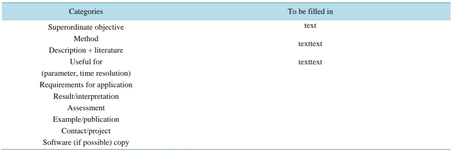
All statistical methods were described in a template which was designed to enable an adequate description of each method (Table 1). This assures that the collected statistical methods are described in a standardized way. Also for this purpose each method is sorted into a prescribed category in order to structure the collection. Be-sides necessary information like description, references and applicability, some important topics are “Require-ments for application”, “Assessment”, and “Example”. These three points particularly help the users to assess the method with regard to their own demands and understand what an outcome may look like and thus make a crucial difference to other collections, statistics books, and guidelines.

Table 1. Template for description of statistical methods.

Categories To be filled in

Superordinate objective Method Description + literature

Useful for (parameter, time resolution) Requirements for application

Result/interpretation Assessment Example/publication

Contact/project Software (if possible) copy

text

texttext

texttext

coastal research, geoscience, ecology, forestry, agriculture, and by different kinds of institutions like universities and other research institutes, federal and regional offices, as well as consulting agencies.

Each method sent to the Working Group (WG) underwent a review process by the members of the working group and an external statistical expert. This comprises a formalistic and content-oriented check. If the descrip-tion did not meet the criteria, the draft was sent back with clear advice what should be added, changed, clarified. Nevertheless, all contributions should be changed as little as possible, so the WG did not correct “the last detail” since the collection was understood as a product “from users to users”. Hence, there may still be some short-comings in the descriptions of the methods, and the descriptions differ in particularity and style. Two external statistics experts reviewed the brochure structuring process. One of them also reviewed each individual method. Examples of the methods are presented in theAnnex.

In the present collection, the order of categories follows the anticipated order of use when evaluating climate data, i.e. the first look at data may probably be via histograms and/or time series. The comparison of model data with observations may lead to the need of a bias-correction. Calculated trends (with methods from time series analysis) must be checked by a suitable significance test. Within each category the methods are ordered accord-ing to their complexity—from simple to complex methods.

Users which may apply the presented statistical methods are provided with additional information concerning the aims and limits of the collection. The editors clearly state that there remains the responsibility of the users to inform themselves on basic knowledge on statistics and check whether the selected method is the right one for the specific question.

4. Selected Examples of Applications

Although the statistics brochure does not claim to be a recipe book “how to combine statistical methods” some hints at the combination of single methods are given in the brochure. This would be highly appreciated by users. But since each problem is unique because of its specific requirements it is not advisable to suggest certain methods or method combinations in general. Nevertheless, four common examples of combining methods for a certain application are described in the introductory chapter. Two examples of rather complex analysis methods are described in the following sections.

4.1. Example “Extreme Value Analysis”

An example for possible ways of extreme event analyses is shown in Figure 1.

In the following, an example for analyzing future extreme wave events in the Baltic Sea is presented. Infor-mation about possible future changes of the wave conditions are needed because they serve as important input parameter for the design of coastal and flood protection structures. The results are moreover used by local au-thorities for the assessment of the future safety and effectiveness of the structures. Significant increases of the future extreme wave heights can lead to increasing loads on the structures, thus different adaptation measures have to be assessed depending on the preferred adaptation strategy (for more details see [20]). The wave dataset that has been analyzed was calculated by using a newly developed hybrid approach that consists of both empiri-cal and numeriempiri-cal methods for the empiri-calculation of the wave conditions based on future projections of wind condi-tions from a regional climate model (COSMO-CLM [21] [22]) considering different future IPCC greenhouse gas emission scenarios (SRES [23]). The associated methods and results have been published in [10] [24].

The wave data were derived within the climate adaptation project RAdOst (Regional Adaptation Strategies for the German Baltic Sea Coast http://klimzug-radost.de/en) and are available for the 20th Century (1960-2000) and 21st Century (2001-2100) on an hourly basis.

Figure 2shows exemplarily the time series of calculated significant wave heights for the 1st realization of the SRES emission scenario A1B near the location of Warnemünde at the German Baltic Sea Coast.

At the beginning of the analyses the time series was tested for linear trends as well as jumps in order to ensure the stationarity and consistency of the underlying data. From the corrected time series (cp. Figure 2) annual maximum values (cp. Block Maxima Method in Figure 1) were selected for different time periods, each con-sisting of 30 years of data. Afterwards, the independence of the sample members was tested and different ex-treme value distribution (EVD) functions like the Generalized Exex-treme Value (GEV) distribution, Weibull, Gumbel and Log-normal function were fitted to the samples by parameter estimation using the Maximum Like-lihood Method (cp. Figure 1).

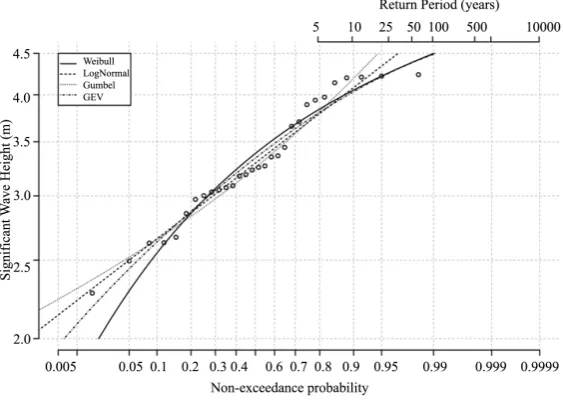
Figure 3shows exemplarily the fitted EVD functions for a sample of 30 years of annual maximum significant wave heights from 2071-2100 and for the 1st realization of the SRES emission scenario A1B near the location of Warnemünde.

For the assessment of the goodness of fit, maximum and root-mean-square differences between the empirical cumulative distribution function (CDF) and theoretical CDFs have been calculated using a modified Kolmo-gorov-Smirnov (K-S) test, consecutively called Lilliefors test. The distribution with the lowest root-mean-square

Figure 1. Possible combinations of methods for analyzing extreme events. The procedures used in the example below are

Figure 2. Time series of calculated significant wave heights (meter) for the 1st realization of the SRES emission scenario A1B near the location of Warnemünde at the German Baltic Sea Coast.

Figure 3. Sample of annual maximum significant wave heights (meter) for the time period 2071-2100 and the 1st realisation of the SRES emission sce-nario A1B near the location of Warnemünde at the German Baltic Sea Coast. The values were plotted log-normally using the plotting position formula (empirical distribution function) by HAZEN.

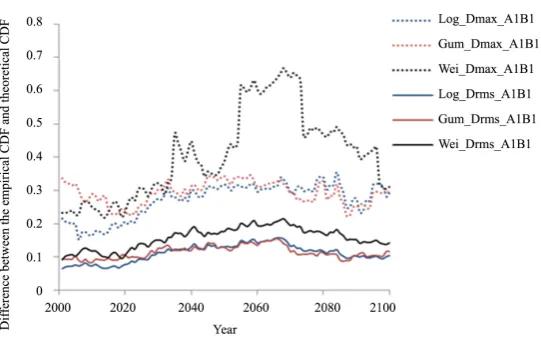
difference was assumed to describe the sample best. InFigure 4 the calculated maximum and root-mean-square differences between the empirical CDF and the theoretical CDFs are shown for the samples consisting of 30 years annual maximum significant wave heights in the 1st realization of the SRES emission scenario A1B (2001-2100) and in the past century C20 (1961-2000) near the location of Warnemünde at the German Baltic Sea Coast.

FromFigure 4 it can be concluded that the Log-normal and Gumbel distribution are showing the lowest root- mean-square differences, thus describing the samples best. In the overall assessment, regarding all emission scenarios used in this study (two realizations each of the scenarios A1B and B1, not shown), the Log-normal function showed the lowest root-mean-square differences in the majority of the comparisons. Another outcome from the overall assessment of the goodness of fit is that the stability or the robustness of the results enhances when taking into account time periods of more than 30 years for the selection of samples.

Figure 4. Maximum and root-mean-square differences (dashed resp. solid lines) between the empirical cumulative distribution function (CDF) and the theoretical CDFs (Weibull, Gumbel and Log-normal) for the 1st realization of the SRES emission scenario A1B (2001-2100) and the past century C20 (1971-2000) near the location of Warnemünde at the German Baltic Sea Coast.

4.2. Example “Ensemble Analysis”

A second challenging task is the analysis and visualization of climate model data using an ensemble of models. This creates a prominent part of the spread of climate projections besides the spread due to different scenarios and climate variability. Both aspects are an inherent part of the uncertainty of climate projections. Presenting the results of an ensemble analysis e.g. to decision makers or other clients in climate service it needs assessment parameters that can be understood. The IPCC reports introduce the term of likelihood [25] to interpret the band-width of results. Other publications define and use a robustness parameter as a measure for the reliability of the results [26]. Innovative maps which show the degree of consensus on the significance of future changes and the sign of the change are presented in [27]. Visualizing uncertainty is not only an actual topic in climate change re-search and service but also in other disciplines which deal with social, demographic, or medical data. Several examples are shown in [28].

In the statistics brochure one chapter is dedicated to the analysis of ensembles with a subchapter presenting their visualization. The presentation of projected climatic changes is an essential part of the communication to stakeholders and decision makers. The message must be clear and comprehensible and include the complexity of climate modeling and the inherent uncertainty.

Two possible ways are shown in Figure 5 andFigure 6, which have been developed for Climate-Fact-Sheets in cooperation with a client http://www.climate-service-center.de/036238/index_0036238.html.en. They origi-nate from the document “How to read a Climate-Fact-Sheet-Instructions for reading and interpretation of the Climate-Fact-Sheets. Climate Service Center, Hamburg, Mai 2013”.

Here, the ensemble analysis is mainly percentile and likelihood analysis. Figure 5 illustrates the scenario in-fluence on the annual cycle of a climate change signal of a parameter, i.e. the difference between projected val-ues in a future time slice and the valval-ues in the reference time slice. Presented is the median of all simulations following a specific scenario, the whole bandwidth based on all scenarios, and the “likely” bandwidth (>66%).

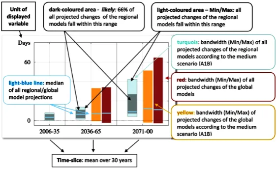
The second example compares the range between the minimum and maximum of different ensembles all available global models for all scenarios, all global models for the A1B scenario, and all available regional models for all scenarios in different time slices.

Since the topic is highly complex the presentations cannot be understood at first glance but working with col-ors, grey areas and info boxes helps users to intuitively understand the context. Note, that the global model data have not been available for the near future period 2006-2035.

5. Conclusions

Figure 5.This figure shows the projected change of the annual cycle in a pa-rameter in % as averaged over the period 2071-2100 compared to the mean of the reference period 1961-1990. Presented are lines of the medians of all global models of all global models of the scenario A1B, and of all regional models, and the regions of likelihood “likely” and the complete bandwidth.

Figure 6. This figure shows the range of the projected change of a parameter averaged over three periods of 30 years 2006-2035, 2036-2065, and 2071- 2100 compared to the mean of the reference period 1961-1990. On the bars the median and the regions of likelihood “likely” and the complete bandwidth

are marked.

recognizing a demand for a compendium on statistical methods among their clients. KLIMZUG offered the great opportunity of testing and applying statistical methods in the process of developing adaptation measures. This effort formed the basis for the collection which is dedicated “from users to users”. The broad scope of KLIMZUG is reflected in the broad range of the statistical methods presented in the compendium. But only the editorial work of categorization and compilation of the methods makes them available for other users. This is a new approach and complements statistical text books as well as statistical software tools. The strengths are standardized presentations of methods, user participation, and editors from different institutions.

ro-bust results. This is e.g. one of the aims of AgMIP (The Agricultural Model Intercomparison and Improvement Project): “Include multiple models, scenarios, locations, crops and participants to explore uncertainty and impact of data and methodological choices” http://www.agmip.org/about-us/objectives/.

The demand for the collection and publication of statistical methods is large, which can be highlighted through the click numbers of the online brochure

http://www.climate-service-center.de/009940/index_0009940.html.de, we count 100 - 200 clicks per month. There is also a link to the brochure on the website of the “Climate Data Guide” of the NCAR (National Center for Atmospheric Research) and UCAR (University Corporation for Atmospheric Research) and funded by the American National Science Foundation

https://climatedataguide.ucar.edu/climate-data-tools-and-analysis/statistical-diagnostic-methods-overview/. The concept of the brochure is a “living document” and the brochure will be updated regularly. The plans for the next update cover the topics: 1) extension of the chapter “Combination of methods”, 2) comparison of dif-ferent methods and assessment of the performance and the differences in the results, 3) extension of the chapter “Ensembles analysis” including visualization.

Acknowledgements

The authors wish to thank the former members of the “Working Group Statistical Methods” (with their former affiliation): Andreas Kochanowski (Helmholtz-Zentrum Geesthacht, Climate Service Center, Hamburg), Oliver Krüger (Helmholtz-Zentrum Geesthacht), Christine Radermacher (Max-Planck-Institutfür Meteorologie, Ham-burg for their contributions. Thanks are also due to Manfred Mudelsee (Climate Risk Analysis) for quality check of the submitted methods and for translating the German Report into English.

References

[1] Hartmann, D.L., Klein Tank, A.M.G., Rusticucci, M., Alexander, L.V., Brönnimann, S., Charabi, Y., Dentener, F.J., Dlugokencky, E.J., Easterling, D.R., Kaplan, A., Soden, B.J., Thorne, P.W., Wild, M. and Zhai, P.M. (2013) Observa-tions: Atmosphere and Surface. In: Stocker, T.F., Qin, D., Plattner, G.-K., Tignor, M., Allen, S.K., Boschung, J., Nauels, A., Xia, Y., Bex, V. and Midgley, P.M., Eds., IPCC, 2013: Climate Change 2013: The Physical Science Basis. Contribution of Working Group I to the Fifth Assessment Report of the Intergovernmental Panel on Climate Change, Cambridge University Press, Cambridge and New York, 1535.

[2] Dore, M.H.I. (2005) Climate Change and Changes in Global Precipitation Patterns: What Do We Know? Environment International, 31, 1167-1181.http://dx.doi.org/10.1016/j.envint.2005.03.004

[3] IPCC (2012) Managing the Risks of Extreme Events and Disasters to Advance Climate Change Adaptation. In: Field, C.B., Barros, V., Stocker, T.F., Qin, D., Dokken, D.J., Ebi, K.L., Mastrandrea, M.D., Mach, K.J., Plattner, G.-K., Allen, S.K., Tignor, M. and Midgley, P.M., Eds., A Special Report of Working Groups I and II of the Intergovernmental Panel on Climate Change, Cambridge University Press, Cambridge and New York, 582.

[4] Giorgi, F., Jones, C., et al. (2009) Addressing Climate Information Needs at the Regional Level: The CORDEX Framework. WMO Bulletin, 58, 175-183.

[5] WMO (2011) Guide to Climatological Practices, WMO-No. 100. 3rd Edition, World Meteorological Organization, Geneva.

[6] Zwiers, F.W. and von Storch, H. (2004) On the Role of Statistics in Climate Research. International Journal of Clima-tology, 24, 665-680. http://dx.doi.org/10.1002/joc.1027

[7] Mudelsee, M. (2010) Climate Time Series Analysis: Classical Statistical and Bootstrap Methods. Atmospheric and Oceanographic Sciences Library, 42.http://dx.doi.org/10.1007/978-90-481-9482-7

[8] UNFCCC (2008) Compendium on Methods and Tools to Evaluate Impacts of, and Vulnerability and Adaptation to, Climate Change.

http://unfccc.int/adaptation/nairobi_work_programme/knowledge_resources_and_publications/items/2674.php

[9] Lu, X. (2011) Applying Climate Information for Adaptation Decision-Making—A Guidance and Resource Document, National Communications Support Programme (NCSP).

http://www.undp.org/content/undp/en/home/librarypage/environment-energy/low_emission_climateresilientdevelopme nt/applying-climate-information-for-adaptation-decision-making/

[11] Mudersbach, C., Bender, J., Kelln, V. and Jensen, J. (2013) Analysing Flood Frequencies at the Elbe River. Do Recent Extreme Events Affect Design Levels? 6th International Conference on Water Resources and Environment Research (ICWRER), Koblenz, 3-7June 2013, 346-362.

[12] Hoffmann, P., Krueger, O. and Schlünzen, K.H. (2012) A Statistical Model for the Urban Heat Island and Its Applica-tion to a Climate Change Scenario. InternaApplica-tional Journal of Climatology, 32, 1238-1248.

http://dx.doi.org/10.1002/joc.2348

[13] Hoffmann, P. and Schlünzen, K.H. (2013) Weather Pattern Classification to Represent the Urban Heat Island in Pre-sent and Future Climate. Journal of Applied Meteorology and Climatology, 52, 2699-2714.

http://dx.doi.org/10.1175/JAMC-D-12-065.1

[14] Schoetter, R., Grawe, D., Hoffmann, P., Kirschner, P., Grätz, A. and Schlünzen, K.H. (2013) Impact of Local Adapta-tion Measures and Regional Climate Change on Perceived Temperature. Meteorologische Zeitschrift, 22, 117-130.

http://dx.doi.org/10.1127/0941-2948/2013/0381

[15] Wilbya, R.L. and Dawson, C.W. (2013) The Statistical DownScaling Model: Insights from One Decade of Application. International Journal of Climatology, 33, 1707-1719. http://dx.doi.org/10.1002/joc.3544

[16] Apata, T.G. (2012) Effects of Global Climate Change on Nigerian Agriculture: An Empirical Analysis. CBN Journal of Applied Statistics, 2, 31-50.

[17] Coles, S. (2001) An Introduction to Statistical Modeling of Extreme Values. Springer Series in Statistics, Springer- Verlag, London. http://dx.doi.org/10.1007/978-1-4471-3675-0

[18] Reiss, R.D. and Thomas, M. (2007) Statistical Analysis of Extreme Values: With Applications to Insurance, Finance, Hydrology and Other Fields (Google eBook). Springer Science & Business Media, Berlin.

[19] Arns, A., Wahl, T., Haigh, I.D., Jensen, J. and Pattiaratchi, C. (2013) Estimating Extreme Water Level Probabilities: A Comparison of the Direct Methods and Recommendations for Best Practice. Coastal Engineering, 81, 51-66.

[20] Fröhle, P., Schlamkow, C., Dreier, N. and Sommermeier, K. (2011) Climate Change and Coastal Protection: Adapta-tion Strategies for the German Baltic Sea Coast. In: Schernewski, G., Hofstede, J. and Neumann, T., Eds., Global Change and Baltic Coastal Zones, Coastal Research Library-Series, Vol. 1, Springer, Dordrecht, 103-116.

http://dx.doi.org/10.1007/978-94-007-0400-8_7

[21] Rockel, B., Will, A. and Hense, A. (2008) The Regional Climate Model COSMO-CLM. Meteorologische Zeitschrift,

17, 347-348. http://dx.doi.org/10.1127/0941-2948/2008/0309

[22] Lautenschlager, M., Keuler, K., Wunram, C., Keup-Thiel, E., Schubert, M., Will, A., Rockel, B. and Boehm, U. (2009) Climate Simulation with CLM. Climate of the 20th Century Run No. 1-3, Scenario A1B Run No.1-2, Scenario B1 Run No.1-2, Data Stream 3: European Region MPI-M/MaD. World Data Center for Climate.

[23] Nakićenović, N., Alcamo, J., Davis, G., de Vries, B., Fenhann, J., Gaffin, S., Gregory, K., Grübler, A., Jung, T.Y., Kram, T., La Rovere, E.L., Michaelis, L., Mori, S., Morita, T., Pepper, W., Pitcher, H., Price, L., Raihi, K., Roehrl, A., Rogner, H.H., Sankovski, A., Schlesinger, M., Shukla, P., Smith, S., Swart, R., van Rooijen, S., Victor, N. and Dadi, Z. (2000) Emissions Scenarios. A Special Report of Working Group III of the Intergovernmental Panel on Climate Change. Cambridge University Press, Cambridge and New York.

[24] Dreier, N., Schlamkow, C., Fröhle, P. and Salecker, D. (2013) Changes of 21st Century’s Average and Extreme Wave Conditions at the German Baltic Sea Coast Due to Global Climate Change. In: Conley, D.C., Masselink, G., Russell, P.E. and O’Hare, T.J., Eds., Proceedings 12th International Coastal Symposium (Plymouth, England), Journal of Coastal Research, Special Issue No. 65.

[25] IPCC (2013) Climate Change 2013: The Physical Science Basis. In: Stocker, T.F., Qin, D., Plattner, G.K., Tignor, M., Allen, S.K., Boschung, J., Nauels, A., Xia, Y., Bex, V. and Midgley, P.M., Eds., Contribution of Working Group I to the Fifth Assessment Report of the Intergovernmental Panel on Climate Change, Cambridge University Press, Cam-bridge and New York, 1535.

[26] Knutti, R. and Sedláček, J. (2013) Robustness and Uncertainties in the New CMIP5 Climate Model Projections. Nature Climate Change, 3, 369-373. http://dx.doi.org/10.1038/nclimate1716

[27] Tebaldi, C., Arblaster, J.M. and Knutti, R. (2011) Mapping Model Agreement on Future Climate Projections. Geo-physical Research Letters, 38, L23701. http://dx.doi.org/10.1029/2011GL049863

[28] Spiegelhalter, D., Pearson, M. and Short, I. (2011) Visualizing Uncertainty about the Future. Science, 333, 1393-1400.

Annex: Method Examples

(category)

Time series analysis

Trend estimation

Method Running mean

Description + literature

Calculation of running 10- and 11-year averages as well as running 30- and 31-year averages, respectively, from transient time series of simulated climate parameters. (Note: If the central point

of the chosen running time interval is considered, usage of 11- and 31-year averages is useful.) Useful for (parameter, time

resolution) Arbitrary variables in monthly, seasonal and yearly resolution.

Requirements for application Sufficiently long, gap-free time series.

Result/interpretation

Rendering the time series as running 10- or 11-year means allows to visualize the decadal variability. Rendering the time series as running 30- or 31-year means allows to determined the

bandwidth of the climate change.

Assessment Simple, fast analysis and visualization.

Example/publication

Jacob, D., Göttel, H., Kotlarski, S., Lorenz, P., Sieck, K. (2008): Klimaauswirkungen und Anpassung in Deutschland: Erstellung regionaler Klimaszenarien für Deutschland mit dem

Klimamodell REMO. Forschungsbericht 20441138 Teil 2, i.A. des UBA Dessau Jacob, D., Bülow, K., Kotova, L., Moseley, C., Petersen, J., Rechid, D.: Regionale Klimasimulationen für Europa und Deutschland-in Vorbereitung

Example 1: Projected changes in winter temperature in the Hamburg metropolitan area as simulated with REMO and CLM, compared with the reference period 1971-2000; plotted as running 11-year

means.

Example 2: Projected changes in winter temperature in the Hamburg metropolitan area as simulated with REMO and CLM, compared with the reference period 1971-2000; plotted as running 31-year

means, also shown yearly values for various scenarios and runs (grey).

Contact/project Diana Rechid, MPI für Meteorologie, [email protected]

Superordinate objective (category) Time series analysis

Method Structural time series analysis, maximum likelihood method

Description + literature

The Gaussian (normal), Gumbel and Weibull probability density functions are described by means of 2 time-dependent parameters (mean and standard deviation)

Trömel, S. (2004):

Statistische Modellierung von Klimazeitreihen, Dissertation, J.W. Goethe Universität Frankfurt am Main,2004.

Useful for (parameter, time resolution) Monthly mean temperature, monthly mean precipitation total

Requirements for application Long, gap-free time series of at least 100 years length

Result/interpretation Trends in mean and standard deviation

Assessment Application of method requires the describability of the time series values by

means of a probability density function (Kolmogorov–Smirnov test)

Example/publication

Bülow, K. (2010): Zeitreihenanalyse von regionalen Temperatur- und

Niederschlagssimulationen in Deutschland, Dissertation, Uni-Hamburg, Berichte zur Erdsystem Forschung 75,2010.

Trömel, S. and C.-D. Schönwiese (2007): Probability change of extreme precipitation observed from 1901 to 2000 in Germany, Theor. Appl. Climatol.,87, 29-39.

Contact/project

Katharina Bülow, Bundesamt für Seeschifffahrt und Hydrographie [email protected]

KLIWA

Superordinate objective (category) Significance tests

Method Bootstrap hypothesis test

Description + literature Bootstrapping is a resampling method. On basis of a single sample, the test is repeated on parametrically or nonparametrically obtained resamples, and a distribution of the test statistic determined (null distribution)

Ususally the test statistic obtained on the sample is compared with the null distribution. This leads to the test significance by comparing the sample-statistic with quantiles of the null distribution.

Climate Time Series Analysis, Mudelsee,2010, pp. 91-94

Useful for (parameter, time resolution) You use bootstrap methods when the theoretical distribution of the statistic of interest is unknown or if no parametric method is available.

Requirements for application Determination of the null distribution depends on the problem at hand.

It is important that the determination of the null distribution has to preserve the original properties of the data generating process (e.g., autocorrelation). For that aim, bootstrap adaptations, such as block bootstrap resampling, can be employed.

Result/interpretation Significance of a hypothesis test (which guides you whether or not to accept the null hypothesis).

Assessment On the one hand, this method delivers results that are independent of strong

assump-tions (positive aspect), but the implementation and application may be difficult (nega-tive). Depending on concept of the bootstrap method and the sample size, this method may be rather computing-intensive.

Example/publication Signifikance test of correlations

Contact/project Oliver Krüger, Helmholtz-Zentrum Geesthacht, Institut für Küstenforschung,

Superordinate objective (category) Extreme value analysis

Method Nonstationary peaks over threshold

Description + literature

Selecting extremes in climatology may sometimes be done more realistically by allowing for a time-dependent “background”, on which a time-dependent variability acts. This nonstationary situation leads then naturally to a time-dependent threshold, in contrast to a stationary situation with a constant threshold.

The method should perform the estimation of the time-dependent background in a robust manner, that is, unaffected by the presence of the assumed extremes. Therefore you use the running me-dian (calculated over the points inside a running window) for nonparametric background or trend estimation, and not the running mean. Analogously, you use the running median of absolute distances to the median (MAD), and not the running standard deviation for variability estimation. Cross-validation techniques offer a guide for selecting the number of window points by optimiz-ing the tradeoff between bias and variance.

Mudelsee, M. (2006) CLIM-X-DETECT: A Fortran 90 program for robust detection of extremes against a time-dependent background in climate records. Computers and Geosciences 32:141-144.

Useful for (parameter, time reso-lution)

All parameters at any temporal resolution.

Note that high time resolution may result in a strong autocorrelation, which has to be considered in the selection of the number of window points (i.e., more window points have to be used com-pared to an autocorrelation-free situation).

Requirements for application

Homogeneity and representativeness of the data. In the case of autocorrelated data, the cross- validation guideline may be less informative and other numbers of window points have to be tried.

Result/interpretation Sample for extreme value analysis (Generalized Pareto distribution, inhomogeneous Poisson process)

Assessment

The challenge of the nonstationary POT method consists in selecting the threshold and the num-ber of window points. Cross-validation guides may help, but it is mandatory to “play” with the data and study the sensitivity of the results in dependence of the selected analysis parameters (threshold, number of window points).

Example/publication

The original paper (Mudelsee 2006) explains the method and describes the Fortran 90 software CLIM-X-DETECT. This analysis type has been applied to a number of climate change analyses, for example, on observed and modelled wildfires 1769-2100 (Girardin and Mudelsee, 2008) or hurricane proxy data 1000-1900 from a lake sediment core (Besonen et al., 2008).

Besonen, M.R., Bradley, R.S., Mudelsee, M., Abbott, M.B., Francus, P. (2008) A 1000-year, annually-resolved record of hurricane activity from Boston, Massachusetts. Geophysical Re-search Letters 35:L14705 (doi:10.1029/2008GL033950).

Girardin MP, Mudelsee M (2008) Past and future changes in Canadian boreal wildfire activity. Ecological Applications 18:391-406.

Mudelsee M (2010) Climate Time Series Analysis: Classical Statistical and Bootstrap Methods. Springer, Dordrecht,474pp.

Contact/project

Manfred Mudelsee