A New Approach of Solving Linear Fractional Programming Problem (LFP) by Using Computer Algorithm

(1)

http://dx.doi.org/10.4236/ojop.2015.43010

A New Approach of Solving Linear

Fractional Programming Problem

(LFP) by Using Computer

Algorithm

Sumon Kumar Saha1_{, Md. Rezwan Hossain}2_{, Md. Kutub Uddin}3_{, Rabindra Nath Mondal}4

1_{Department of Applied Mathematics, Gono Bishwabidyalay (University), Dhaka, Bangladesh} 2_{Department of Business Development, Allcare Limited, Dhaka, Bangladesh}

3_{Department of Mathematics, University of Dhaka, Dhaka, Bangladesh} 4_{Department of Mathematics, Jagannath University, Dhaka, Bangladesh}

Email: [email protected], [email protected], [email protected]

Received 3 June 2015; accepted 1 September 2015; published 4 September 2015

This work is licensed under the Creative Commons Attribution International License (CC BY). http://creativecommons.org/licenses/by/4.0/

Abstract

In this paper, we study a new approach for solving linear fractional programming problem (LFP) by converting it into a single Linear Programming (LP) Problem, which can be solved by using any

type of linear fractional programming technique. In the objective function of an LFP, if β is

nega-tive, the available methods are failed to solve, while our proposed method is capable of solving such problems. In the present paper, we propose a new method and develop FORTRAN programs to solve the problem. The optimal LFP solution procedure is illustrated with numerical examples and also by a computer program. We also compare our method with other available methods for solving LFP problems. Our proposed method of linear fractional programming (LFP) problem is very simple and easy to understand and apply.

Keywords

Linear Programming, Linear Fractional Programming Problem, Computer Program

1. Introduction

(2)

for linear programming to the ratio of linear functions or to the case of the ratio of quadratic functions in such a situation. All these problems are fragments of a general class of optimization problems, termed in the literature as fractional programming problems. This field of LFP was developed by Hungarian mathematician Matros [1] [2] in 1960. Several methods are proposed to solve this problem. Charnes and Kooper [3] have proposed their method depended on transforming this (LFP) to an equivalent linear program, they say the feasible region X

is nonempty and bounded, cx+α and ax+β do not vanish simultaneously in S then they used the variable transformation y=tx t, ≥0 in such a way that dt+ =β γ where γ ≠0 is a specified number and transform LFP to an LP problem. Multiplying the numerator and denominator and the system of inequalities by t and

, 0

y=tx t≥ , they obtain two equivalent LP problems and name them as EP and EN. If EP or EN has an optimal solution and other is inconsistence, then LFP also has an optimal solution. If any of the two problems EP or EN is unbound, then LFP is also unbound. So if the first problem is not unbound, one needs to solve the other. That’s why one needs to solve two LPs by Big-M or two-phase simplex method, which is a very lengthy process. On the other hand, the simplex type algorithm is introduced by Swarup [4] and Swarup, Gupta and Mohan [5]. In that method one needs to compute ∆ =j Z2

(

cj−Zj1

) (

−Z1 dj−Zj2

)

in each step and continues this process

until the value of ∆j satisfying the required condition. We see that it has to deal with the ratio of two linear

functions, that’s why its computational process is complicated and also when the constraints are not in canonical form then it becomes lengthy. Another method is called updated objective function method derived from Bitran and Novaes [6] is used to solve this linear fractional program by solving a sequence of linear programs only re-computing the local gradient of the objective function. But to solve a sequence of problems sometimes may need many iterations and at some cases say, dx+ ≥β 0 and cx+ <α 0 ∀ ∈x S, Bitran-Novaes method is failed. Singh [7] in his paper makes a useful study about the optimality condition in fractional programming. Tantawy [8] develops a technique with the dual solution. Hasan and Acharjee [9] also develop a method for solving LFP by converting it into a single LP, but for the negative value of β, their method fails. Tantawy [10] develops another technique for solving LFP which can be used for sensitivity analysis. Effati and Pakdaman [11] propose a method for solving the interval-valued linear fractional programming problem. Pramanik et al. [12] develops a method for solving multi-objective linear plus linear fractional programming problem based on Tay-lor Series approximation.

In this paper, our intent is to develop a new technique for solving any type of LFP problem by converting it into a single linear programming (LP) problem because at some cases in the denominator and numerator when β is negative, available methods are failed to solve the linear fractional problem. We also develop a FOR- TRAN computer program for solving it and analyze the solution by numerical examples.

2. Mathematical Formulation of LP and LFP

The mathematical expression of a general linear programming problem is as follows:

Maximize (or Minimize) 1

n

j j

j

Z c x

=

∑

Subject to

{

}

1

, , ; 1, 2, ,

n

ij j i

j

a x b i m

=

≤ = ≥ =

∑



0; 0

x≥ b≥

where one and only one of the signs (≤, =, ≥) holds for each constraint and the sign may vary from one con-straint to another. Here cj

(

j=1, 2,,n

)

are called profit (or cost) coefficients, xj

(

j=1, 2,,n

)

are called

decision variables. The set of feasible solution to the linear programming problem (LP) is

(

) (

)

{

T T

}

1, 2, , : 1, 2, ,

n

n n

S= x x  x x x  x ∈R and

(

x x1, 2,,xn

)

T. The set S is called the constraints set, feasible

set or feasible regionof (LP).

In matrix vector notation the above problem can be expressed as: Maximize (or Minimize) Z=cx

Subject to Ax

(

≤ = ≥, ,

)

b

0; 0

x≥ b≥

(3)

The mathematical formulation of an LFP (in matrix vector notation) is as follows:

Maximize Z cx dx

α β + =

+ Subject to Ax

(

≤ = ≥, ,

)

b

0; 0

x≥ b≥

where A is an m n× matrix, x is an n×1 column vector, b is an m×1 column vector and c is a 1×n row vector, m

b∈R ; _{x c d}, , _∈_Rn_;α β ∈_, _R_.

2.1. Solving LFP by Our Method

If c≠0 and d≠0, we assume that the feasible reason S=

{

x∈Rn:Ax≤b x, ≥0

}

is nonempty and bounded and the denominator dx+ ≠β 0.

We convert the LFP into an LP in the following way assuming that β ≠0. Case I: β >0

For objective function,

(

)

(

)

c d x

cx cx

Z

dx dx dx

β α

α α α α α

β β β β β β β

−

+ +

= = − + = +

+ + +

( )

H y Iy J

∴ = +

where, I cβ dα

β −

= , y x

dx β

=

+ , J α β =

For constraint, Ax≤b

1 Ay

b yd

β

⇒ ≤

−

b y

Aβ bd

⇒ ≤ +

(

Aβ bd y

)

b

⇒ + ≤

Ky L

∴ ≤

where K =Aβ+bd L, =b

So the new LP is: Maximize H y

( )

=Iy+J Subject to Ky≤L, y≥0

2.2. Calculation for the Unknown Variable of the LFP

From the above LP, we get y x dx β

= +

1 y x

dy

β ∴ =

−

This is our required optimal solution. Putting the value of x in the original objective function, we can get the optimal value.

Case II: β <0, α≥0 For objective function,

cx Z

dx

α β + =

(4)

(

)

(

)

1 1

c d x

Z cx dx c x

Z cx dx c d x d x

α β

α β α

α β α β β

+ + − ′ ′

+ + + − +

⇒ = = =

′ ′

− + − + − + + +

where, α′= −α β β , ′= +α β and c′= +c d d , ′= −c d

Same as above procedure, we have

( )

H′ y =I y′ +J′

where, I cβ dα

β ′ ′− ′ ′ ′ =

′ ,

x y

d x β

=

′ + ′, J α β ′ ′ =

′,

( )

1 1 Z

H y

Z

+

′ =

− For constraints, following the same procedure as above, we get

K y′ ≤L′

where K′=Aβ′+bd L′ ′, =b

Case III: β <0, α<0 For objective function:

cx cx

Z

dx dx

α α

β β

− − +

= =

− − +

Same as above procedure, we have

( )

1 1 1

H y =I y+J

where, 1

d c

I α β

β −

= , y x

dx β

=

− + , J1 α β =

For constraints, following the same procedure as above, we get

1 1

K y≤L

where K1=Aβ−bd L, 1=b.

3. Algorithm

If β >0 then

; ; ; ;

c d x

I y J K A bd L

dx b

β α α

β β

− _← _← _← ₊

+ ←

←

( )

;

H y ← +Iy J for all Ky≤L&y≥0; else if β <0 &α ≥0 then

; ;c c d d; c d;

α′← −α β β′← +α β ′← + ′← −

; ; ;

c d x

I y J

d x

β α α

β β β

′ ′− ′ ′ ′

′← ← ′←

′ ′ + ′ ′

; K′←Aβ′+bd′ L′←b

( )

;

H′ y ←I y′ +J′ for all K y′ ≤L′&y≥0;

( )

_{( )}

1

1 H y H y

H y

′ +

←

′ −

else

1 ; ; 1 ; 1 ; 1

d c x

I y J K A bd L b

dx

α β α _β

β β β

−

← ← ← ← − ←

− +

( )

1 1

(5)

4. Numerical Examples

Here we illustrate some numerical examples to demonstrate our method. Example 1:

Minimize 1 2

1 2

2 2

3 4

x x

Z

x x

− + +

=

+ +

Subject to − +x1 x2≤4

1 2

2

1 2

2 14

6 , 0

x x

x x x

+ ≤

≤ ≥

Solution: Here we have, c= −

(

2,1 ,

)

d=

( )

1, 3 ,α =2,β =4,A1= −

(

1,1 ,

) ( )

A2 2,1 ,A3=

( )

0,1 ,b1=4,b2=14,

3 6

b = , where A b1, 1 is related to the first constraint, A b2, 2 is related to the second constraint and A b3, 3 is related to the third constraint. So, we have the new objective function.

Minimize

( )

(

) ( )

1

1 2

2

4 2,1 2 1, 3 2 5 1 1

4 4 2 2 2

y

H y y y

y

− −

   

=_ _{  }+ = − − +

 

Now for the first constraint,

(

)

( )

1

2

1,1 4 4 1, 3 y 4

y

 

− + ≤

 _{  }

 

2 1 4 y

⇒ ≤

For the second constraint,

( )

1

2

4 2,1 14 1, 3 y 14

y

 

+ ≤

 _{  }

 

1 2

11y 23y 7

⇒ + ≤

For the third constraint,

( ) ( )

1

2

4 0,1 6 1, 3 y 6

y

 

+ ≤

 _{  }

 

1 2

3y 11y 3

⇒ + ≤

Converting the LP in standard form we have

Maximize

( )

1 2

5 1 1

min

2 2 2

T y = − H y = y + y −

Subject to 2 1 1 4 y + =s

1 2 2

11y +23y +s =7

1 2 3

3y +11y +s =3

1, 2, ,1 2 0 y y s s ≥

(6)

Table 1. Initial table for Example 1.

CΒ

J

C 5

2

1

2 0 0 0

b

Basis y1 y2 s1 s2 s3

0 s1 0 1 1 0 0

1 4

0 s2 11 23 0 1 0 7

0 s3 3 11 0 0 1 3

j j j

c = −c E 5

2

1

[image:6.595.91.541.611.666.2]

2 0 0 0

Table 2.Final table for Example 1.

CΒ

J

C 5

2

1

2 0 0 0

b

Basis y1 y2 s1 s2 s3

0 s1 0 1 1 0 0

1 4 5

2 y1 1

23

11 0

1

11 0

7 11

0 s3 0

52

11 0

3 11

− 1 12

11

j j j

c = −c E 0 52

11

− 0 5

22

− 0

So we have, 1 7 11

y = , y2=0

Now

(

)

(

)

( )(

1 2

)

_{( )}

( )

1 2

7 28

, 0 4 , 0

, 11 11

, 7, 0

11 7

1 1, 3 ,

1 1, 3 , 0

4 11

y y x x

y y

β _ _ _ _

= = = =

− ₋  

 

 

Putting this value in the original objective function, we have

Min 2 7 0 2 12

7 3 0 4 11

Z=− × + + = −

+ × +

Now, we solve the above problem by computer program. Output:

Minimum value of the Objective Function = −1.090909. X1 = 7.000000;

X2 = 0.000000.

We see that our hand calculation result and computer oriented solution is the same. This shows that our com-puter program is correct.

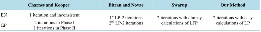
Charnes and Kooper Bitran and Novae Swarup Our Method

EN 1 iteration and inconsistent

1st_{LP-2 iterations}

2nd_{LP-2 iterations} 2 iterations with clumsy _{calculations of LFP} 2 iterations with easy _{calculations of LP}

EP 2 iterations in Phase I

1 iterations in Phase II

Example 2:

Maximize 1 2

1 2

2 3

1

x x

Z

x x

+ =

(7)

Subject to x1+x2≤3

1 2

2 3

, 0

x x

x x

+ ≤

≥

Solution: Here we have, c=

( )

2, 3 ,d =

( )

1,1 ,α =0,β= −1,A1 =

( )

1,1 ,b1 =3,A2 =

( )

1, 2 ,b2 =3, where A b1, 1 is related to the first constraint and A b2, 2 is related to the second constraint.

Now, α′= −1,β′=1,c′=

( )

3, 4 ,d′=

( )

1, 2 So, we have the new objective function

Maximize

( ) ( ) ( )( )

1

( )

2

3, 4 1 1, 2 1 1

1 1

y H y

y

− − −

   

′ =_ _{  }+

 

( )

4 1 6 2 1 H′ y = y + y −

( )

1

2

1,1 1 3 1, 2 y 3 y

 

+ ≤

 _{  }

 

1 2

4y 7y 3

⇒ + ≤

For the first constraint,

( )

1

2

1, 2 1 3 1, 2 y 3 y

 

+ ≤

 _{  }

 

1 2

4y 8y 3

⇒ + ≤

Converting the LP in standard form we have Maximize H′

( )

y =4y1+6y2−1

Subject to 4y1+7y2+ =s1 3

1 2 2

4y +8y +s =3

1, 2, ,1 2 0 y y s s ≥

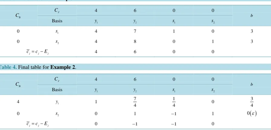
[image:7.595.73.504.109.495.2]

Now we get the following tables (Table 3 and Table 4):

CΒ

J

C 4 6 0 0

b

Basis y1 y2 s1 s2

0 s1 4 7 1 0 3

0 s2 4 8 0 1 3

j j j

c = −c E 4 6 0 0

Table 4.Final table for Example 2.

CΒ

J

C 4 6 0 0

b

Basis y1 y2 s1 s2

4 y1 1

7 4

1

4 0

3 4

0 s2 0 1 −1 1 0( )ε

j j j

[image:7.595.90.538.504.720.2]

(8)

So we have, 1 3 4

y = , y2=0

Now

(

)

(

)

( )(

1 2

)

_{( )}

( )

1 2

3 3

, 0 1 , 0

, ₄ ₄

, 3, 0

1 3

1 1, 2 ,

1 1, 2 , 0 4 4

y y x x

y y

β′ _ _ _ _

= = = =

− ₋  

 

 

Maximum 2 3 3 0 3

3 0 1 Z = × + × =

+ −

By using computer technique we get the following result. Output:

Maximum value of the Objective Function = 3.000000. X1 = 3.000000;

X2 = 0.000000.

Note: This problem cannot be solved by any available method because the value of β is negative. Example 3:

Maximize 1 2

1 2

6 5 4

2 3 8

x x Z x x − − = + −

Subject to 2x1−2x2≤3

1 2

3 2 2

, 0

x x

x x

+ ≤

≥

Solution: Maximize 1 2 1 2

1 2 1 2

6 5 4 6 5 4

2 3 8 2 3 8

x x x x

Z

x x x x

− − − + +

= =

+ − − − +

Subject to 2x1−2x2≤3

1 2

3 2 2

, 0

x x

x x

+ ≤

≥

Here we have, c= −

(

6, 5 ,

)

d = − −

(

2, 3 ,

)

α =4,β =8,A1=

(

2, 2 ,−

)

b1 =3,A2 =

( )

3, 2 ,b2 =2, where A b1, 1 is related to the first constraint and A b2, 2 is related to the second constraint.

So we have the new objective function

Maximize

( ) (

) (

)

1

1 2

2

6, 5 8 2, 3 4 4 13 1

5

8 8 2 2

y

H y y y

y − − − −     =_ _{  }+ = − + +    

(

) (

)

1

2

2, 2 8 2, 3 3 y 3

y   − + − − ≤  _{  }  _{ } 1 2

10y 25y 3

⇒ − ≤

For the second constraint,

( ) (

)

1

2

3, 2 8 2, 3 2 y 2

y   + − − ≤  _{  }     1 2 1 2

20 10 2

10 5 1

y y

⇒ + ≤

Converting the LP in standard form, we have

Maximize

( )

1 2

13 1

5

2 2

(9)

Subject to 10y1−25y2+ =s1 3

1 2 2

10y +5y +s =1

1, 2, ,1 2 0 y y s s ≥

Now we get the following tables (Table 5 and Table 6):

CΒ

J

C −5 13 2 0 0

b

Basis y1 y2 s1 s2

0 s1 10 −25 1 0 3

0 s2 10 5 0 1 1

j j j

c = −c E −5 13 2 0 0

Table 6. Final table for Example 3.

CΒ

J

C −5 13 2 0 0

b

Basis y1 y2 s1 s2

0 s1 40 0 1 5 8

13 2 y2 2 1 0 1 5 1 5

j j j

c = −c E −18 0 0 −13 10

So we have y1=0, 2

1 5 y =

Now,

(

)

(

)

(

1 2

)(

)

₍

₎

( )

1 2

1 8

0, 8 0,

, 5 5

, 0,1

8 1

1 2, 3 ,

1 2, 3 0,

5 5 y y

x x

y y

β _ _ _ _

= = = =

− − −  

− − −  

 

Maximum 6 0 5 1 4 9

2 0 3 1 8 5

Z = × − × − =

× + × −

Using computer program, we get the following result. Output:

Maximum value of the Objective Function = 1.800000. X1 = 0.000000;

X2 = 1.000000.

Example 4: Production Problem of a Certain Industry.

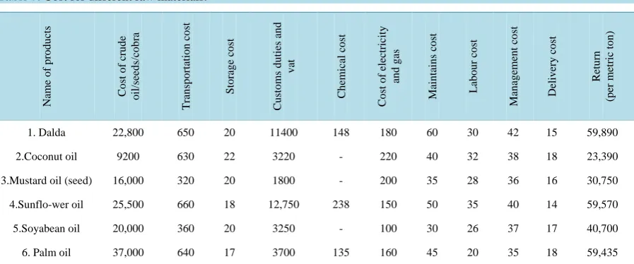
Suppose an industry has Tk. 3,00,00,000/= by which it can produce six different products Palm oil, Coconut oil, Mustard oil, Soyabean oil, Sunflower oil and Dalda. The net refined oil from per metric ton cobra, master seeds, sunflower seeds, palm crude oil, soyabean crude oil are respectively 300 kg, 400 kg, 400 kg, 980 kg, 970 kg. The industry has some production loss for palm oil and soyabean oil, which are respectively 2% and 3%. The industry has a fixed establishment cost is Tk. 5,00,000. The management of industry wishes to produce maxi-mum 600 metric tons different types of oil. The cost for different raw materials to produce per metric ton crude oil/ seed/cobra in taka as follows (Table 7).

(10)

Maximum investment for crude oil/seeds/cobra is Tk. 20,000,000/-; Maximum investment for transportation is Tk. 5,00,000/-;

Maximum investment for storage is Tk. 15000/-;

Maximum investment for customs duties and vat is Tk. 6,000,000/-; Maximum investment for chemicals is Tk. 55,000/-;

Maximum investment for electricity and gas is Tk. 120,000/-; Maximum investment for maintains is Tk. 30,000/-;

[image:10.595.89.538.213.400.2]

Maximum investment for labor is Tk. 10,000/-; Maximum investment for management is Tk. 25,000/-.

Table 7.Cost for different raw materials.

N am e of pr oduc ts C os t of c rude o il/s eed s/co b ra T ran sp o rtatio n co st Sto rag e co st C us tom s dut ie s a nd v at C h em ical co st Co st o f electr ic ity an d g as M ain tain s co st L abour c os t M an ag em en t co st Deliv er y co st R etu rn (p er m etr ic to n )

1. Dalda 22,800 650 20 11400 148 180 60 30 42 15 59,890

2.Coconut oil 9200 630 22 3220 - 220 40 32 38 18 23,390

3.Mustard oil (seed) 16,000 320 20 1800 - 200 35 28 36 16 30,750

4.Sunflo-wer oil 25,500 660 18 12,750 238 150 50 35 40 14 59,570

5.Soyabean oil 20,000 360 20 3250 - 100 30 26 37 17 40,700

6. Palm oil 37,000 640 17 3700 135 160 45 20 35 18 59,435

The objective is to maximize the ratio of return to investment. This leads to a linear fractional program as shown below.

Formulation of Example 4.

The three basic steps in constructing an LFP model are as follows:

Step 1. Identify the unknown variables to be determined (decision variables) and represent them in terms of algebraic symbols.

Step 2. Identify all the restrictions or constraints in the problem and express them as linear equations or in-equalities, which are linear functions of the unknown variables.

Step 3. Identify the objective or criterion and represent it as a ratio of two linear functions of the decision va-riables, which is to be maximized (or minimized).

Now we shall formulate the above problem as follows: Step 1. Identify the decision variables.

For this problem the unknown variables are the metric tons of refined oil produced for different product. So, let

1

x = The metric tons of dalda has to be refined;

2

x = The metric tons of coconut oil has to be refined;

3

x = The metric tons of mustard oil has to be refined;

4

x = The metric tons of sunflower oil has to be refined;

5

x = The metric tons of soyabean oil has to be refined;

6

x = The metric tons of palm oil has to be refined. Step 2. Identify the constraints.

In this problem constraints are the limited availability of found for different purposes as follows:

1) Since the management of industry wishes to produce maximum 600 metric tons different types of oil, so we have

1 2 3 4 5 6

(11)

2) Since the industry has maximum investment for crude oil/ seeds/ cobra is Taka 2,00,00,000/-, so we have

1 2 3 4 5 6

22800x +9200x +16000x +25500x +20000x +37000x ≤20000000

3) Since the industry has maximum investment for transportation is Taka 500,000/-, so we have

1 2 3 4 5 6

650x +630x +320x +660x +360x +640x ≤500000

4) Since the industry has maximum investment for storage is Taka 15,000/-, so we have

1 2 3 4 5 6

20x +22x +20x +18x +20x +17x ≤15000

5) Since the industry has maximum investment for customs duties and vat is Taka 6,000,000/-, so we have

1 2 3 4 5 6

11400x +3220x +1800x +12750x +3250x +3700x ≤6000000

6) Since the industry has maximum investment for chemical cost is Taka 6,000,000/-, so we have

1 4 6

148x +238x +135x ≤50000

7) Since the industry has maximum investment for electricity and gas is Taka 120,000/-, so we have

1 2 3 4 5 6

180x +220x +200x +150x +100x +160x ≤120000

8) Since the industry has maximum investment for maintains is Taka 30,000/-, so we have

1 2 3 4 5 6

60x +40x +35x +50x +30x +45x ≤30000

9) Since the industry has maximum investment for labor is Taka 200,000/-, so we have

1 2 3 4 5 6

30x +32x +28x +35x +26x +20x ≤200000

10)Since the industry has maximum investment for delivery is Taka 10,000/-, so we have

1 2 3 4 5 6

15x +18x +16x +14x +17x +18x ≤10000

11)Since the industry has maximum investment for management is Taka 25,000/-, so we have

1 2 3 4 5 6

42x +38x +36x +40x +37x +35x ≤25000

We must assume that the variables x ii, =1, 2,, 6 are not allowed to be negative. That is, we do not make negative quantities of any product.

Step 3. Identify the objective function.

In this case, the objective is to maximize the ratio of total return and investment by different crops. That is

( )

1 2 3 4 5 6

59890 23390 30750 59750 40700 59435

Maximize

500000 35345 13420 18455 39455 23840 41770

x x x x x x

F x

x x x x x x

+ + + + +

=

+ + + + + +

Now we have expressed our problem as a mathematical model. Since the objective function is the ratio of re-turn to investment and all of the constraints functions are linear, the problem can be modeled as the following LFP model:

( )

1 2 3 4 5 6

59890 23390 30750 59750 40700 59435

Maximize

500000 35345 13420 18455 39455 23840 4177

x x x x x x

F x

x x x x x x

+ + + + +

=

+ + + + + +

Subject to 0.3x1+0.4x2+0.4x3+0.98x4+0.97x5+0.98x6≤600

1 2 3 4 5 6

228005x +9200x +16000x +25500x +20000x +37000x ≤20000000

1 2 3 4 5 6

650x +630x +320x +660x +360x +640x ≤500000

1 2 3 4 5 6

20x +22x +20x +18x +20x +17x ≤15000

1 2 3 4 5 6

11400x +3220x +1800x +12750x +3250x +3700x ≤6000000

1 4 6

148x +238x +135x ≤50000

1 2 3 4 5 6

(12)

1 2 3 4 5 6

60x +40x +35x +50x +30x +45x ≤30000

1 2 3 4 5 6

30x +32x +28x +35x +26x +20x ≤200000

1 2 3 4 5 6

15x +18x +16x +14x +17x +18x ≤10000

1 2 3 4 5 6

42x +38x +36x +40x +37x +35x ≤25000

1, 2, 3, 4, 5, 6 0 x x x x x x ≥

The problem consists of 6 decision variables and 11 constraints. To solve it by hand calculations it involves 17 variables and 11 constraints, which cannot be accommodated in available size of papers. Moreover, in real life, there may be some problems which may be involved with hundreds of constraints and variables and hence these cannot be solved by hand calculations. To overcome difficulties one has to require computer oriented solu-tions. Now, applying the computer program, we have obtained the following solusolu-tions.

Output:

X1 = 22.774542; X2 = 0.000000; X3 = 0.000000; X4 = 0.000000; X5 = 11.660869; X6 = 0.000000.

Maximum value of the Objective Function = 1.655239.

5. Comparison

In this section, we compare our method with all other available methods and we find that our method is better than any other available method. The reasons are as follows:

• We can solve any type of linear fractional programming problems by this methodology. • We can easily transfer the LFP problem into a LP problem.

• Its computational steps are so easy from other methods.

• In this method, we need to solve one LP but by other methods one needs to solve more than one LP, and thus our method saves valuable time.

• The final result converges quickly in this method. • In this method there is one restriction that is β ≠0.

• In some cases of the denominator and numerator say, dx+ >β 0 and cx+ <α 0 ∀ ∈x X , where Btran- Novaes method fails and for the negative value of β all other existing methods are also failed, but our me-thod is able to solve the problem very easily.

• Using computer program, we get the optimal solution of the LFP problem very quickly.

6. Conclusion

In this paper, we have provided a new method for solving linear fractional programming problem (LFPP). While all other existing methods are failed in the case of negative value of β, but our method can solve the problem vary easily. At first we transform the LFP problems into an LP and then solve it by using simplex method. Then we develop a computer program for solving such problems, and verify that our computer program is correct. We illustrate a number of numerical examples to demonstrate our method. After that we compare our method with other existing methods. We further conclude that the proposed concept will be helpful in solving real-life prob-lems involving linear fractional programming probprob-lems in agriculture, production planning, financial and cor-porate planning, health care, hospital management, etc. Thus our newly developed method with computer pro-gram saves time and energy and is easy to apply.

References

[1] Martos, B. (1960) Hyperbolic Programming, Publications of the Research Institute for Mathematical Sciences. Hunga-rian Academy of Sciences, 5, 386-407.

(13)

http://dx.doi.org/10.1002/nav.3800110204

[3] Charnes, A. and Cooper, W.W. (1962) Programming with Linear Fractional Functions. Naval Research Logistics Quarterly, 9, 181-186. http://dx.doi.org/10.1002/nav.3800090303

[4] Swarup, K. (1964) Linear Fractional Functional Programming. Operations Research, 13, 1029-1036.

http://dx.doi.org/10.1287/opre.13.6.1029

[5] Swarup, K., Gupta, P.K. and Mohan, M. (2003) Tracts in Operation Research. 11th Edition.

[6] Bitran, G.R. and Novaes, A.J. (1973) Linear Programming with a Fractional Objective Function. Operations Research,

21, 22-29. http://dx.doi.org/10.1287/opre.21.1.22

[7] Sing, H.C. (1981) Optimality Condition in Fractional Programming. Journal of Optimization Theory and Applications,

33, 287-294. http://dx.doi.org/10.1007/BF00935552

[8] Tantawy, S.F. (2007) A New Method for Solving Linear Fractional Programming problems. Australian Journal of Ba-sic and Applied Science, 1, 105-108.

[9] Hasan, M.B. and Acharjee, S. (2011) Solving LFP by Converting It into a Single LP. International Journal of Opera-tions Research, 8, 1-14.

[10] Tantawy, S. (2008) An Iterative Method for Solving Linear Fraction Programming (LFP) Problem with Sensitivity Analysis. Mathematical and Computational Applications, 13, 147-151.

[11] Effati, S. and Pakdaman, M. (2012) Solving the Interval-Valued Linear Fractional Programming Problem. American Journal of Computational Mathematics, 5, 51-55. http://dx.doi.org/10.4236/ajcm.2012.21006