Heart Rate Variability Analysis and Pathological Detection

Heart Rate Variability Analysis and Pathological

Detection

Payal Patial

LPU, Punjab, India.

Kawaldeep Singh

LPU, Punjab, India.

ABSTRACT

In order to measure the mortality in the patients suffering from the heart disease we use the term HRV that i.e. Heart Rate Variability. Estimation methods as Parametric and Non-Parametric are used in the analysis of Heart Rate Variability but Heart Rate Variability requires the specific capabilities which are not provided by either of these. The term EMD i.e. Empirical Mode Decomposition adaptively estimates the IMF i.e. Intrinsic Mode Function of the nonlinear and nonstationary signal. The IMF obtained from the EMD is used for the analyses of the HRV latencies of Healthy subjects and of Congestive Heart Failure subjects. In this paper we have considered the 15 Congestive Heart Failure patients, 20 healthy young control patients and 20 healthy old control patients. After finding the IMF from EMD we have calculated the average periods, absolute power, normalised power and cumulative power and concerned plots are drawn for the comparison of the considered subjects. The results obtained shows that the HRV of healthy subjects rises rapidly to its maximum response as compared to the HRV of the pathological subjects. This fact can be used as a promising approach in clinical practise for the screening of specific risk group.

General Terms

HRV Analysis using EMD, Pathological Detection.

Key-words

Empirical Mode Decomposition, Heart Rate Variability, Average Period, Absolute Power, Normalised and Cumulative Power.

1. INTRODUCTION

The phenomenon that focuses on the oscillation in the interval between consecutive heartbeats as well as the oscillations between consecutive instantaneous heart rates is known as the Heart rate variability. Heart Rate Variability has become the conventionally accepted term to describe variations of both instantaneous heart rate and RR intervals. The results obtained from HRV data are capable of portraying physiological condition of the patient moreover they are an important indicator of cardiac pathologies. Variations in heart rate are clinically linked to various lethal arrhythmias, congestive heart failure, hypertension, organ transplant, coronary artery disease, tachycardia, bradycardia, diabetes and neuropathy etc.

Heart is influenced and para-sympathetic activities of the autonomic nervous system. Sympathetic activities i.e. fight and flight it accelerates the heart rate where as parasympathetic activity i.e. rest and digest it decelerates the heart rate. Sympathovagal balance gives the influence of both the branches of autonomic nervous system and this balance is reflected in HRV and HRV is non invasive measure of autonomic nervous system. EMD is given by Huang et al and showed that it is a method of decomposing the nonlinear non stationary multi component signal. The components which results from EMD are known as IMF. Algorithm used for defining EMD has no analytical formulation implementation. Decomposition of the signal is understood easily by the experimental investigation of it rather than the analytical results. As EMD is fully data dependent and adaptive in nature, hence it is highly efficient method for decomposition of any nonlinear and non stationary signals [6].

2.

EMPIRICAL

MODE

DECOMPOSITION

There are few assumptions we made for EMD which are as follows.

 The signal has at least two extrema’s: one maxima and one minima.

 Characteristic time scale must be equal to the time lapse between the extrema.

 Differentiation once or more than once is done in order to reveal the extrema, it the data is totally devoid of extrema and have some inflection points [6].

Net final result i.e. the signal is obtained from the integration of IMF components. Decomposition of data is done accordingly after identifying the intrinsic oscillatory modes.

3. INTRINSIC MODE FUNCTION

The results obtained after the decomposition the process consists of components known as IMF. IMF has two conditions which have to be satisfied.

 The no. of extrema and zero crossing must be either equal to or differ by at most 1.

In each cycle of IMF, zero crossing involves only one mode of oscillation with no complex riding waves.

4. MATERIAL AND METHODOLOGY

Dataset for HRV analysis is obtained from Physionet Fantasia Database; we have considered the ECG signal for concerned subject and obtained the R peaks for HRV analysis. We have considered three different groups as.

 20 Healthy young subjects.

 20 Healthy old subjects.

 15 Congestive Heart Failure.

4.1 QRS Detection

In order to get the RR-Interval we need to obtain the R peaks in the concerned signal. For R peaks we undergo through QRS detection and there various methods associated with it. In this paper Pan and Tompkin method for QRS Detection is applied. Ri - Ri-1 intervals are

obtained from the R peaks of the concerned ECG signal and also known as NN interval. Variation in these RR intervals is knows as Heart Rate Variability [10] [12] [13].

4.2 EMD Methodology

 EMD is used to estimate the local time scales of HRV signal decomposition and consists of various steps.

 Signal to be analysed = s(t); auxiliary variable = x; variable = k; it is the no. of estimated IMF which is set to zero.

 Apply spline to the upper and lower extrema. It will give us the upper and lower envelope.

 Find the arithmetic mean between the upper and lower envelope. It is called the average envelope (m).

 IMF is estimated by the difference between mean of upper and lower envelop and the signal.

IMF = x – m or h = x – m

 There are various conditions associated with IMF in case if h does not satisfy those conditions then repeat the steps for x, m, h.

 If h satisfies the conditions required for h then save IMF as Ck and k is kth component.

 Mean square error between two consecutive IMF. ck-i

and ck and the value obtained is compared with

stopping condition.

 Partial residue (rk) is estimated as difference between

a previous partial residue (rk-1 and ck) and assigned to

dummy variable (x) and repeat the steps.

 After stopping condition, the final residue (rfinal) can

be estimated as the difference between s(k) and sum of all IMFs.

After sifting process the original signal s(t) can be represented as

………...…... (1)

Where n = no. of IMF, ck= kth IMF, rfinal=final residue [15]

[16].

4.3 Time Domain HRV Measures

4.3.1 Using EMD

The power of the nth IMF is computed as given in:

= …...………. (2) where, Cn = nth IMF and j=1….N samples.

The average period (mean period) of the IMF, Cnis given

as:

………... (3)

where, dist = distance between the first and last zero crossings and Zc = number of zero crossings.

4.3.2 Using RR-Intervals

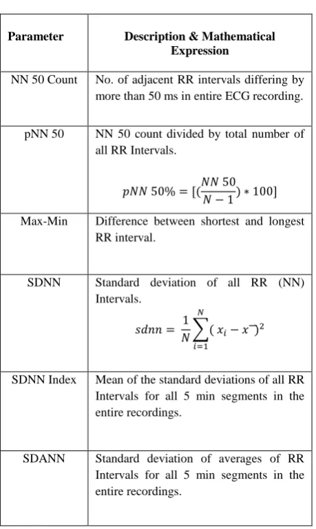
Time domain parameters are obtained using the RR-Intervals [3] [4] [11]. The associated formulae with the frequency and time domain parameters are given in Table 1 as follows.

Table 1. Time domain parameters of HRV

Parameter Description & Mathematical

Expression

NN 50 Count No. of adjacent RR intervals differing by more than 50 ms in entire ECG recording.

pNN 50 NN 50 count divided by total number of all RR Intervals.

Max-Min Difference between shortest and longest RR interval.

SDNN Standard deviation of all RR (NN) Intervals.

SDNN Index Mean of the standard deviations of all RR Intervals for all 5 min segments in the entire recordings.

RMSSD Root mean square of the difference of successive RR Intervals.

SDSD Standard deviation of differences between adjacent RR (NN) Intervals.

HRV Index Total number of all RR Intervals divided by amplitude of all RR Intervals.

4.4 Frequency Domain HRV Measures

4.4.1 Using RR-Intervals

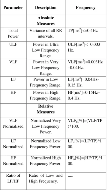
Frequency domain parameters are obtained using the RR-Intervals [3] [4] [11]. The associated formulae with the frequency and time domain parameters are given in Table 2 as follows.

Table 2. Frequency domain parameters of HRV

Parameter Description Frequency

Absolute Measures

Total Power

Variance of all RR intervals.

TP[ms2]<=0.4Hz

ULF Power in Ultra Low Frequency

Range.

ULF[ms2]<=0.003 Hz.

VLF Power in Very Low Frequency

Range.

VLF[ms2]=0.003Hz –0.04Hz.

LF Power in Low Frequency Range.

LF[ms2 ]=0.04Hz-0.15 Hz.

HF Power in High Frequency Range.

HF[ms2]=0.15Hz– 0.4 Hz.

Relative Measures

VLF Normalized

Normalized Very Low Frequency

Power.

VLFn[%]=(VLF/TP

)*100.

LF Normalized

Normalized Low Frequency Power.

LFn[%]=(LF/TP)*1

00.

HF Normalized

Normalized High Frequency Power.

HFn[%]=(HF/TP)*1

00.

Ratio of LF/HF

Ratio of Low and High Frequency.

...

5. RESULTS

5.1 Using EMD

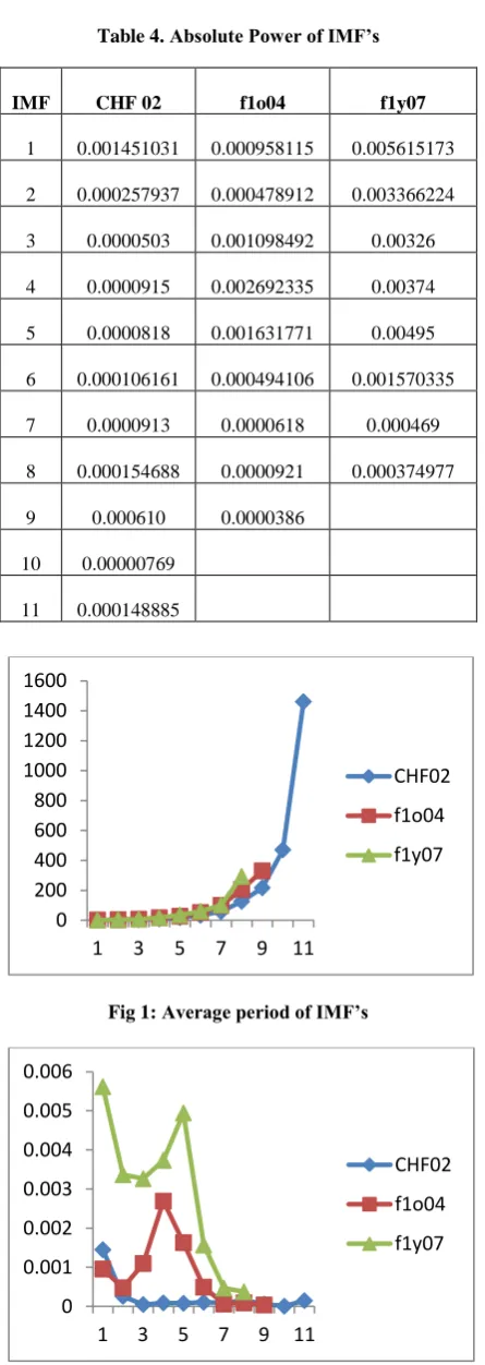
The EMD method is applied to half hour duration i.e. for 450000 samples as recording of 1 hour consists of 900000 samples. HRV measurements of 20 healthy young subjects, 20 healthy old subjects and 15 congestive heart failure subjects have been considered and method is applied to them. The EMD method decomposes the signals into IMF effectively. Here, we have considered three signals as CHF02, f1o04 and f1y07, and results shows that CHF02 consists of 11 IMF, f1o04 consists of 9 IMF and f1y07 consists of 8 IMF. The additional component in CHF patient’s HRV was due to the latencies present in the signal. Further we have calculated the average period (tn)

and absolute power (Vn) of the IMF of the concerned

signals using eqn. 2 and 3 respectively and calculated values of average period (tn) and absolute power (Vn) given

in table 3 and 4. Plotting the average periods (tn) of IMFs

against its IMF number gives an exponential graph as shown in Fig. 1. According to the plot average period (tn)

of IMFs of CHF 02 subject is significantly lower in value and the rate of increase w.r.to IMFs also smaller compared to healthy controls. The computed absolute power (Vn) of

IMFs for the 3 subjects was presented in Fig. 2. For healthy young control subject f1y07 the absolute power (Vn) was high in all IMFs. For healthy old control subject

f1o04 the power is less compared to healthy young in all IMFs except in IMF4 and dominates all the other IMFs. But for CHF 02 the absolute powers (Vn) of all IMFs were

completely suppressed and found in lower range. Here are the Table 3 and Fig 1 representing the Average period of the IMF’s of the signals and Table 4 and Fig 2 showing the Absolute Power of the IMF’s of signals.

Table 3. Average period of IMF’s

IMF CHF 02 f1o04 f1y07

1 1.538181818 1.54829134 1.949811794

2 2.484466835 3.424778761 3.969309463

3 4.672985782 7.03196347 7.701492537

4 8.618075802 16.63043478 16.97802198

5 17.63855422 26.89285714 34.65116279

6 32.75555556 51.5862069 60.3627564

7 57.43137255 98.86666667 101.5714286

8 125.8571429 206.3333333 292.75234

9 216.3333333 329.6666667

10 470

Table 4. Absolute Power of IMF’s

IMF CHF 02 f1o04 f1y07

1 0.001451031 0.000958115 0.005615173

2 0.000257937 0.000478912 0.003366224

3 0.0000503 0.001098492 0.00326

4 0.0000915 0.002692335 0.00374

5 0.0000818 0.001631771 0.00495

6 0.000106161 0.000494106 0.001570335

7 0.0000913 0.0000618 0.000469

8 0.000154688 0.0000921 0.000374977

9 0.000610 0.0000386

10 0.00000769

11 0.000148885

Fig 1: Average period of IMF’s

Fig 2: Absolute Power of IMF’s

5.2 Using RR-Intervals

5.2.1 Time Domain Parameters

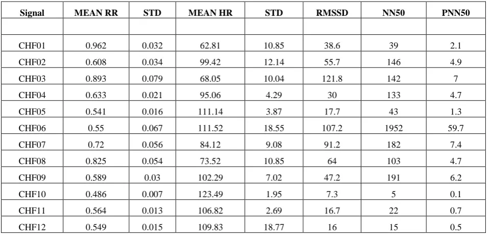
The estimation of HRV can be done by the time domain measures. The HRV was measured manually from the mean R-R interval in time domain and its standard deviation is measured on short-term 5 minute ECG segment. On the basis of these methods either the heart rate or each QRS complex or the RR intervals between successive normal complexes are determined and then analyzed. But the recordings for a longer period of 24 hours sometimes lead to complex statistical time-domain analysis.

These statistical parameters may be derived from direct measurements of the RR intervals or from the differences between RR intervals. The simplest variable to calculate is square root of variance i.e. the standard deviation of the NN interval (SDNN). Time domain HRV variables are detailed in Table 1 and calculated values of time domain parameters is given in Table 6.

5.2.2 Frequency Domain Parameters

Frequency Domain Analysis includes the frequency measures on the ECG data and frequency measures involve the spectral analysis of HRV. If the spectrum estimate is calculated from this irregularly time sampled signal, additional harmonic components appear in the spectrum, and then interpolation is required. The RR interval signal is then interpolated before the spectral analysis so that they can recover an evenly sampled signal from the irregularly sampled event series. The HRV spectrum contains the high frequency (0.18 to 0.4 Hz) component, which is due to respiration and the low frequency (0.04 to 0.15 Hz) component that appears due to both the vagus and cardiac sympathetic nerves. Ratio of the low-to-high frequency spectra is used as an index of parasympathetic sympathetic balance. Frequency domain HRV variables are detailed in Table 2, calculated values of frequency domain parameters is given in Table 5 and plot is given in Fig 3.

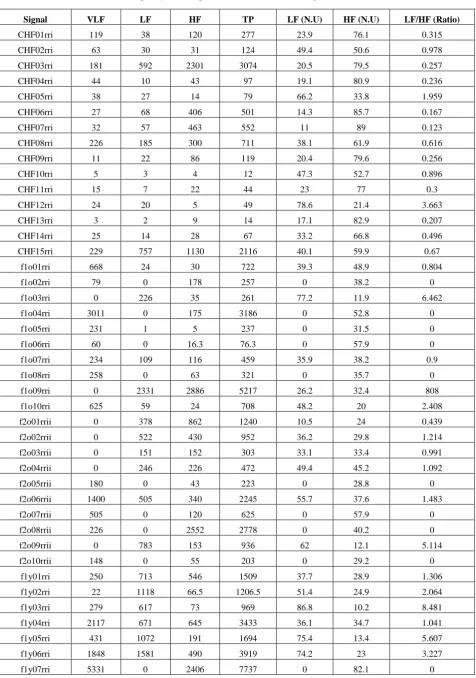
The non parametric frequency domain parameters for the RR-Intervals have been calculated. The use of computationally efficient algorithms such as Fast-Fourier Transform, the HRV signal is decomposed into its individual spectral components and their intensities, using Power Spectral Density (PSD) analysis [14]. These spectral components are then grouped into three distinct bands: very-low frequency (VLF), low frequency (LF) and high frequency (HF).

The cumulative spectral power in the LF and HF bands and the ratio of these spectral powers (LF/HF) has demonstrable physiological relevance in healthy and disease states. Changes in the LF band spectral power (0.04– 0.15Hz) reflect a combination of sympathetic and parasympathetic ANS outflow variations, while changes in the HF band spectral power (0.15–0.40Hz) reflect vagal modulation of cardiac activity. The LF/HF power ratio is used as an index for assessing sympatho-vagal balance. The calculated LF/HF values are given in Table 6 & plot for it is shown in Fig 3.

0 200 400 600 800 1000 1200 1400 1600

1 3 5 7 9 11

CHF02

f1o04

f1y07

0 0.001 0.002 0.003 0.004 0.005 0.006

1 3 5 7 9 11

CHF02

f1o04

Table 5 Frequency domain parameters (Parametric) using RR-Intervals

Signal VLF LF HF TP LF (N.U) HF (N.U) LF/HF (Ratio)

CHF01rri 119 38 120 277 23.9 76.1 0.315

CHF02rri 63 30 31 124 49.4 50.6 0.978

CHF03rri 181 592 2301 3074 20.5 79.5 0.257

CHF04rri 44 10 43 97 19.1 80.9 0.236

CHF05rri 38 27 14 79 66.2 33.8 1.959

CHF06rri 27 68 406 501 14.3 85.7 0.167

CHF07rri 32 57 463 552 11 89 0.123

CHF08rri 226 185 300 711 38.1 61.9 0.616

CHF09rri 11 22 86 119 20.4 79.6 0.256

CHF10rri 5 3 4 12 47.3 52.7 0.896

CHF11rri 15 7 22 44 23 77 0.3

CHF12rri 24 20 5 49 78.6 21.4 3.663

CHF13rri 3 2 9 14 17.1 82.9 0.207

CHF14rri 25 14 28 67 33.2 66.8 0.496

CHF15rri 229 757 1130 2116 40.1 59.9 0.67

f1o01rri 668 24 30 722 39.3 48.9 0.804

f1o02rri 79 0 178 257 0 38.2 0

f1o03rri 0 226 35 261 77.2 11.9 6.462

f1o04rri 3011 0 175 3186 0 52.8 0

f1o05rri 231 1 5 237 0 31.5 0

f1o06rri 60 0 16.3 76.3 0 57.9 0

f1o07rri 234 109 116 459 35.9 38.2 0.9

f1o08rri 258 0 63 321 0 35.7 0

f1o09rri 0 2331 2886 5217 26.2 32.4 808

f1o10rri 625 59 24 708 48.2 20 2.408

f2o01rrii 0 378 862 1240 10.5 24 0.439

f2o02rrii 0 522 430 952 36.2 29.8 1.214

f2o03rrii 0 151 152 303 33.1 33.4 0.991

f2o04rrii 0 246 226 472 49.4 45.2 1.092

f2o05rrii 180 0 43 223 0 28.8 0

f2o06rrii 1400 505 340 2245 55.7 37.6 1.483

f2o07rrii 505 0 120 625 0 57.9 0

f2o08rrii 226 0 2552 2778 0 40.2 0

f2o09rrii 0 783 153 936 62 12.1 5.114

f2o10rrii 148 0 55 203 0 29.2 0

f1y01rri 250 713 546 1509 37.7 28.9 1.306

f1y02rri 22 1118 66.5 1206.5 51.4 24.9 2.064

f1y03rri 279 617 73 969 86.8 10.2 8.481

f1y04rri 2117 671 645 3433 36.1 34.7 1.041

f1y05rri 431 1072 191 1694 75.4 13.4 5.607

f1y06rri 1848 1581 490 3919 74.2 23 3.227

f1y08rri 881 562 150 1593 70.3 18.8 3.737

f1y09rri 0 1416 99 1515 78.6 5.5 14.247

f1y10rri 725 767 290 1782 64.9 24.5 2.648

f2y01rrii 240 435 510 1185 37.5 44 0.853

f2y02rrii 2056 733 796 3585 46.3 50.3 0.921

f2y03rrii 821 0 278 1099 0 71.9 0

f2y04rrii 286 161 103 550 53 3.8 1.5

f2y05rrii 454 1057 788 2299 47 35 1.342

f2y06rrii 391 1509 146 2046 96.4 9.3 10.362

f2y07rrii 810 878 1031 2719 49 57.5 0.852

f2y08rrii 306 952 934 2192 36.5 35.8 1.019

f2y09rrii 0 988 1621 2609 19.6 32.1 0.609

f2y10rrii 4031984 15482 829 4048295 91.1 4.9 18.683

Fig 3: Plot of LF/HF Ratio

Table 6 Time domain parameters using RR-Intervals

Signal MEAN RR STD MEAN HR STD RMSSD NN50 PNN50

CHF01 0.962 0.032 62.81 10.85 38.6 39 2.1

CHF02 0.608 0.034 99.42 12.14 55.7 146 4.9

CHF03 0.893 0.079 68.05 10.04 121.8 142 7

CHF04 0.633 0.021 95.06 4.29 30 133 4.7

CHF05 0.541 0.016 111.14 3.87 17.7 43 1.3

CHF06 0.55 0.067 111.52 18.55 107.2 1952 59.7

CHF07 0.72 0.056 84.12 9.08 91.2 182 7.4

CHF08 0.825 0.054 73.52 10.85 64 103 4.7

CHF09 0.589 0.03 102.29 7.02 47.2 191 6.2

CHF10 0.486 0.007 123.49 1.95 7.3 5 0.1

CHF11 0.564 0.013 106.82 2.69 16.7 22 0.7

CHF12 0.549 0.015 109.83 18.77 16 15 0.5

0 1 2 3 4 5 6

1 2 3 4 5 6 7 8 9 10 11 12 13 14 15 16 17 18 19 20

CHF02

f1o04

CHF13 0.614 0.012 97.85 3.73 16.2 28 1

CHF14 0.776 0.019 77.51 6.23 22 40 1.7

CHF15 0.581 0.038 103.98 7.19 55.8 199 6.4

f1o01 0.991 0.028 60.64 1.94 15.7 5 0.3

f1o02 1.03 0.036 58.44 4.35 55.7 14 0.8

f1o03 0.974 0.025 61.69 1.77 21.3 23 1.2

f1o04 1.16 0.072 52.03 4.39 49.6 166 10.7

f1o05 1.058 0.022 56.76 1.4 11.6 1 0.1

f1o06 1.179 0.028 50.96 1.8 43.5 18 1.2

f1o07 0.981 0.039 61.29 2.75 40.8 95 5.2

f1o08 0.818 0.031 73.53 3.46 30.1 39 1.8

f1o09 1.412 0.142 43.25 7.16 190.8 470 36.9

f1o10 0.855 0.038 70.47 3.47 24.5 27 1.3

f2o01 0.901 0.094 67.8 10.68 152.2 236 11.8

f2o02 1.091 0.054 55.16 3.64 74 83 5

f2o03 1.053 0.032 57.1 2.61 44 59 3.5

f2o04 1.024 0.03 58.68 2.11 32.2 82 4.7

f2o05 0.789 0.027 76.22 5.28 29.4 32 1.4

f2o06 1.331 0.063 45.29 3.37 58.4 278 20.6

f2o07 1.198 0.035 50.14 1.93 34.4 60 4

f2o08 0.972 0.119 63.39 13.33 196.1 265 14.3

f2o09 1.123 0.06 53.98 8 52.9 27 1.7

f2o10 0.772 0.027 78.02 3.76 35.2 20 0.9

f1y01 0.784 0.065 77.15 7.33 73.3 853 37.2

f1y02 0.992 0.067 60.85 4.54 68.4 770 42.5

f1y03 0.914 0.044 65.92 3.36 29 153 7.8

f1y04 1.306 0.09 46.35 6.21 106.2 900 65.3

f1y05 0.98 0.059 61.6 4.77 48.6 352 19.2

f1y06 1.027 0.086 59.28 12.5 66.9 536 30.6

f1y07 1.157 0.13 52.94 7.54 113.2 937 60.3

f1y08 0.967 0.06 62.42 4.55 44.9 430 23.1

f1y09 0.852 0.061 71 5.75 35.8 280 13.3

f1y10 0.794 0.06 76.15 6.19 53.6 493 21.8

f2y01 0.0871 0.054 69.23 4.77 68.3 703 34

f2y02 1.071 0.087 56.6 5.18 78.6 616 48.8

f2y03 1.047 0.034 57.47 3.83 36.5 134 7.8

f2y04 0.797 0.035 75.57 3.91 29.5 59 2.6

f2y05 0.767 0.047 78.57 6.66 62.1 24 1

f2y06 982 0.041 61.3 5.43 32.8 104 5.7

f2y07 1.086 0.071 55.67 4.05 78.3 85.4 51.5

f2y08 0.983 0.079 61.65 7.79 99.1 1089 59.5

f2y09 0.797 0.109 77.37 15.06 163.9 746 33

6. DISCUSSION

A practical method for analyzing the HRV latencies is presented in this study using the database of CHF patients and healthy subjects. It is observed that the latencies of HRV signal effectively discriminates the healthy subjects and congestive heart failure subjects significantly. The opted method of EMD was applied to half an hour HRV measurement of healthy controls and congestive heart failure patients and a good discrimination of the two groups were obtained by it. The EMD method estimates the local time scales adaptively which reflects the intrinsic properties of the signal. This feature makes the healthy systems to reach its maximum response much earlier and makes the system more adaptive than congestive heart failure patients. Moreover, the LF/HF ratio by using frequency domain parametric approach has been calculated. Results are showing that the CHF patients has low LF/HF ratio as compared to the healthy subjects. It represents that the CHF patients have less sympatho-vagal balance of sympathetic and parasympathetic autonomic nervous system.

7. CONCLUSION

The common hypothesis is that the human cardiovascular system is a highly complex adaptive system and that the complexity of its behaviour allows for the broadest range of adaptive responses. The proposed technique is simple and adaptive method to analyze the complex HRV signal. The fastness in reaching maximum response of the healthy system represents its more adaptiveness for particular level of input and the slowness in reaching maximum response (more latency) of CHF subjects represents the system’s inability to respond quickly for various levels of inputs. The estimate of LF/HF ratio also helps in finding the sympatho-vagal balance of sympathetic and parasympathetic autonomic nervous system. This fact makes the method a promising approach to be applied in clinical practice as a screening test for specific risk-groups.

8. ACKNOWLEDGMENTS

I am very thankful to Mr. Kawaldeep Singh Chandok for his kind guidance and support in completion of this paper. And I am also to thankful to my friend Suraj Bhati for his support and motivation.

9. REFERENCES

[1] Rangayyan R.M., Biomedical Signal Analysis: A Case-study Approach, Wiley–Interscience, New York, 2001.

[2] Reddy, D.C., Biomedical Signal Processing: Principles and Techniques, Tata McGraw-Hill, New Delhi, 2005.

[3] Argyro Kampouraki, George Manis, and Christophoros Nikou, (2009). “Heartbeat Time Series Classification with Support Vector Machines’, IEEE, July 2009.

[4] Marcel STANCIU, Mihaela ALBU, Anatolie BOEV, (2009). “ECG monitoring: A software tool for deriving time and frequency parameters”, IEEE, May 2009.

[5] J. G. Proakis and M. D. G., Digital Signal Processing: Principles, Algorithms, and Applications: Prentice- Hall, 1999.

[6] M.E.S. Chelladurai and N. Kumaravel, 2011. Heart Rate Variability Analysis in Different Age and Pathological Conditions, International Journal of Computer Applications.

[7] Neto, E.P.S., M.A. Custaud, J.C. Cejka, P. Abry and J. Frutoso et al., 2004. Assessment of cardiovascular autonomic control by the empirical mode decomposition. Methods Inf. Med., 43. DOI: 10.1267/METH04010060

[8] Lindsen, J.P. and J. Bhattacharya, 2010. Correction of blink artifacts using independent component analysis and empirical mode decomposition. Psychophysiology, 47.

[9] Feldman, D., T.S. Elton, D.M. Menachemi and R.K. Wexler, 2010. Heart rate control with adrenergic blockade: Clinical outcomes in cardiovascular medicine. Vascular Health Risk Manage, 6. DOI: 10.2147/VHRM.S10358

[10]N. E. Huang, Z. Shen, C. C. Tung, M. C. Wu, H. H. Shih, Q. Zheng, S. R. Long N.- C. Yen, , and H. H. Liu, "The empirical mode decomposition and the Hilbert spectrum for nonlinear and non-stationary time series analysis," Proc. R. Soc. Lond.,1998. [11]Pan J. and Tompkins W. J. A real-time QRS detection

algorithm. IEEE Trans. Biomed. Eng. BME-32. [12]1985. Task force of the European society of

cardiology and the North American society of pacing and electrophysiology. Heart rate variability: standards of measurement, physiological interpretation, and clinical use. Circulation, vol.93, no.5, 1996.

[13]Bansal Dipali, Khan Munna and Salhan A.K. An ECG monitoring system having simple interface with computer capable of real time data transfer. International Conference, Los-Angeles, USA, P1.7, 2007.

[14]Ahlstrom, M. L. and Tompkins W. J. Digital filters for real-time ECG signal processing using microprocessors. IEEE Trans. Biomed. Eng., BME-32, 1985.

[15]Shafqat, K., S.K. Pal, S. Kumari and P.A. Kyriacou, 2009. Empirical Mode Decomposition (EMD). Proceeding of the 31st Annual International Conference of the IEEE EMBS Minneapolis, Sept. 3-6, IEEE Xplore Press, Minneapolis, MN.