Evaluation of normalization procedures for oligonucleotide array data based on spiked cRNA controls

comment

reviews

reports

deposited research

interactions

information

refereed research

Research

Evaluation of normalization procedures for oligonucleotide array

data based on spiked cRNA controls

Andrew A Hill*, Eugene L Brown*, Maryann Z Whitley*, Greg

Tucker-Kellogg*

†

_{, Craig P Hunter}

‡

_{and Donna K Slonim*}

Address: *Department of Genomics, Genetics Institute/Wyeth-Ayerst Research, Cambridge, MA 02140, USA. ‡_{Department of Molecular and} Cellular Biology, Harvard University, Divinity Avenue, Cambridge, MA 02138, USA. †_{Current address: Millennium Pharmaceuticals, One} Kendall Square, Cambridge MA 02139, USA.

Correspondence: Andrew A Hill. E-mail: ahill@genetics.com; Donna K Slonim. E-mail: dslonim@gomez.genetics.com

Abstract

Background: Affymetrix oligonucleotide arrays simultaneously measure the abundances of thousands of mRNAs in biological samples. Comparability of array results is necessary for the creation of large-scale gene expression databases. The standard strategy for normalizing oligonucleotide array readouts has practical drawbacks. We describe alternative normalization procedures for oligonucleotide arrays based on a common pool of known biotin-labeled cRNAs spiked into each hybridization.

Results: We first explore the conditions for validity of the ‘constant mean assumption’, the key assumption underlying current normalization methods. We introduce ‘frequency normalization’, a ‘spike-in’-based normalization method which estimates array sensitivity, reduces background noise and allows comparison between array designs. This approach does not rely on the constant mean assumption and so can be effective in conditions where standard procedures fail. We also define ‘scaled frequency’, a hybrid normalization method relying on both spiked transcripts and the constant mean assumption while maintaining all other advantages of frequency normalization. We compare these two procedures to a standard global normalization method using experimental data. We also use simulated data to estimate accuracy and investigate the effects of noise. We find that scaled frequency is as reproducible and accurate as global normalization while offering several practical advantages.

Conclusions:Scaled frequency quantitation is a convenient, reproducible technique that performs as well as global normalization on serial experiments with the same array design, while offering several additional features. Specifically, the scaled-frequency method enables the comparison of expression measurements across different array designs, yields estimates of absolute message abundance in cRNA and determines the sensitivity of individual arrays.

Published: 21 November 2001

GenomeBiology2001, 2(12):research0055.1–0055.13

The electronic version of this article is the complete one and can be found online at http://genomebiology.com/2001/2/12/research/0055 © 2001 Hill et al., licensee BioMed Central Ltd

(Print ISSN 1465-6906; Online ISSN 1465-6914)

Received: 27 July 2001 Revised: 28 September 2001 Accepted: 17 October 2001

Background

Affymetrix oligonucleotide arrays (referred to here as oligonucleotide arrays) are widely used to measure the abun-dance of mRNA molecules in biological samples [1]. The

array [2]. There is a significant amount of assay noise associ-ated with readouts from oligonucleotide arrays (for example [3,4]). For these arrays we have found additive and multi-plicative noise affecting individual gene readouts (typically 5-20%), as well as multiplicative noise affecting entire arrays (often above 20%). As defined here, normalization attempts to correct for only the latter type of noise. The primary sources of this array-level noise are between-array variation in overall performance (due to inconsistencies in array fabri-cation, staining and scanning), and between-cRNA variation (as independently prepared cRNAs have variable purity and/or fluorescently-labeled mass fractions). Because these sources of variation contribute so significantly to array read-outs, normalization is a critical first step in any analysis of gene expression data.

Most current normalization procedures for oligonucleotide arrays are global approaches, based on normalization of the overall mean or median array intensity to a common stan-dard (for example [5-7]). Spiked stanstan-dards have also been used to normalize cDNA [8] and oligonucleotide [9-11] arrays. All these techniques are inherently linear; there have been recent reports of nonlinear normalizations for cDNA [12], oligonucleotide [13,14] and other [15] arrays. Few detailed comparisons of oligonucleotide-array normalization procedures have been reported, however [13].

For oligonucleotide arrays, the normalization implemented in the Affymetrix GeneChipTM_{software (Affymetrix, Santa}

Clara, CA) is by far the most commonly used (for example [1,16]). In this approach, the mean hybridization intensities (the ‘average differences’ (AD)) of all probe sets on each array are scaled to an arbitrary, fixed level [17]. In the rest of this paper, we refer to this procedure as ‘global normaliza-tion’ or scaled average difference (ADs_{). In practice, there are}

at least three limitations to this method. Of these, the first two relate to the normalization itself, and the last relates to the practical utility of the normalized readouts.

First, global normalization makes no attempt to absolutely quantify mRNA abundances. Readouts are normalized to an arbitrary scale, which may vary from one operator to another or between experiments. In contrast, previous experiments with spiked controls [1] and comparisons with serial analysis of gene expression (SAGE) [18] have shown that array response can be proportional to true transcript abundance, suggesting that absolute quantitation of transcripts is feasi-ble. If sufficiently accurate, such an absolute scale for all array readouts could facilitate comparisons across large, diverse gene expression databases.

Second, global normalization implicitly assumes that the mean expression level of all monitored mRNAs is constant. The validity of this assumption depends on the number and biological characteristics of genes monitored by an array. For smaller arrays that monitor a limited set of mRNAs, this

assumption is invalid and may result in erroneous normal-ization. Ideally, a quantitation method for arrays would be effective even in cases where this ‘constant mean’ hypothesis does not hold.

Third, as typically applied, global normalization does not deal well with transcripts expressed at low copy numbers. In a typical Affymetrix GeneChip assay, many low-abundance transcripts are present at levels below the sensitivity of detection of the array (typically about 1:100,000 mRNAs). Measurements for such mRNAs are not only noisy but are sometimes negative, due to cross-hybridization to mismatch probes [1]. Negative intensity values are meaningless and problematic because they cannot be log-transformed, a manipulation that is a common prelude to downstream analysis of array data. Simply discarding negative values is objectionable as it can lead to missed observations of biolog-ically significant upregulation. An automated normalization method that handles noisy and negative measurements and responds to variable array sensitivity is desirable, especially in a high-throughput setting.

The primary criterion for any alternative to global normal-ization is that it should expand the investigator’s ability to compare diverse array experiments done at different times in different laboratories. In this paper, we describe alterna-tive procedures that seek to quantitate array results in terms of transcripts per unit cRNA. We chose cRNA quantitation because it meets the primary criterion, and for several addi-tional reasons.

First, cRNA quantitation is easily applied to array experi-ments using small amounts of starting total RNA that are difficult to quantitate accurately. Second, the spike reagents described here for cRNA quantitation can be used to specifically monitor the performance of individual arrays. Third, in our experience, the reproducibility, accu-racy and scientific value of cRNA quantitation are at least as good as those of alternative techniques, such as proce-dures to quantitate transcripts per cell, transcripts per mass of input material, transcripts per total RNA or tran-scripts per polyadenylated RNA.

We evaluated two alternatives to the standard global nor-malization scheme which we term ‘frequency’ (F) and ‘scaled frequency’ (Fs_{) normalization. These normalization}

comment

reviews

reports

deposited research

interactions

information

refereed research

simulated data, we compare the reproducibility and accuracy of frequency, scaled frequency and global normalization. Our results suggest that scaled frequency normalization is a useful strategy for oligonucleotide array data and has impor-tant advantages over current approaches.

Results and discussion

A key assumption underlying global normalization is that the mean expression level on an array should be the same for all samples and all arrays. This assumption is distinct from the additional implicit assumption that the fraction of polyadenylated mRNA per total RNA is constant. One can certainly construct special cases where the constant-mean assumption is invalid. One example would be using a small array containing only genes from a single pathway in an experiment that studies variable induction of that pathway. However, it is unclear how well even more general array experiments satisfy this assumption.

To evaluate the constant-mean assumption we examined the coefficient of variation (CV) of the mean expression level of variable-sized mRNA sets across samples covering widely divergent developmental stages of the nematode

Caenorhabditis elegans. We constructed the largest possible

subset of our data that included only matched triplets of the A, B and C array designs (see Materials and methods). The subset comprised 39 chip hybridzations, 13 of each design, covering all developmental stages. This dataset represents a

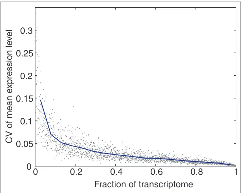
relatively strong test of the constant mean assumption, because very large biological modulation of many mRNAs occurs across the dataset. As the C. elegansarrays monitor around 98% of all predicted C. elegans mRNAs, and the sum of the relative expression levels of all expressed genes must be constant by definition, global normalization is well justi-fied for the dataset as a whole. Thus, the 13 experimental hybridizations of each array design were globally normal-ized, and subsets of the 19,031 total mRNAs monitored by the arrays were selected at random. For each subset, the CV of the mean expression level of the subset across all 13 hybridizations was computed. Subsets ranged in size from 10 to 19,031 genes (0.05% to 100% of this transcriptome) (Figure 1). The CV of the mean expression level is below 7% for any set of mRNAs larger than roughly 10% of the total. As this CV is no larger than the typical contribution of other noise sources in the readout, we conclude that the constant-mean assumption can be supported for arrays that monitor on the order of 20-100% of a transcriptome. This is typical of current commercial arrays for several bacteria, yeast, mouse and human.

Table 1

Spike-in transcript pool

Spiked ATCC Affymetrix Final Final

transcript accession gene concentration concentration

number qualifier (pmol) (ppm)

DAPM 87826 AFFX-DapX-M_at 30 950

DAP5 87827 AFFX-DapX-5_at 10 317

CRE5 87832 AFFX-CreX-5_at 5 158

BIOB5 87825 AFFX-BioB-5_at 2.5 79

BIOD3 87830 AFFX-BioDn-3_at 1.2 38

BIOB3 87828 AFFX-BioB-3_at 0.6 19

CRE3 87835 AFFX-CreX-3_at 0.4 13

BIOC5 87833 AFFX-BioC-5_at 0.3 10

BIOC3 87834 AFFX-BioC-3_at 0.2 6

DAP3 87831 AFFX-DapX-3_at 0.15 5

BIOBM 87829 AFFX-BioB-M_at 0.1 3

Spike-in transcript pool. The 11 spiked transcripts and their final concentrations in the hybridization cocktails are listed. The Affymetrix gene qualifier column indicates the name of the probe set on Affymetrix arrays that monitors each spiked transcript.

Figure 1

When to use mean normalization. The constant-mean assumption adds little noise for array designs with sufficiently large numbers of randomly selected genes. Assuming that the mean expression on arrays in a dataset would indeed be constant for an array monitoring the entire transcriptome, we chose random subsets of genes of each possible size and computed the CV of the mean expression level for hypothetical arrays monitoring just those subsets of genes. For arrays measuring more than about 10% of the genes, the level of variability introduced is not significantly larger than other sources of array variability, so

normalization using the constant-mean assumption is reasonable. With fewer genes, the noise introduced by making this assumption grows dramatically, so other normalization methods may be desirable. Note that if there is bias in the selection of genes on the array, this effect may be much stronger.

0 0.2 0.4 0.6 0.8 1

0 0.05 0.1 0.15 0.2 0.25 0.3

Fraction of transcriptome

CV of mean e

xpression le

v

These results only apply when genes monitored by an array are randomly selected with respect to their expression char-acteristics. The example noted above (all genes on an array from a single pathway) is an extreme case of nonrandom selection. Other common ways of selecting genes for arrays may also violate this assumption, including selection based on matches in specific cDNA libraries.

Nonrandom selection of even large mRNA sets for individual arrays can also lead to between-array inconsistencies in mean expression level. For example, consider the case of two arrays, each monitoring a large, equal percentage (> 20%) of a transcriptome, where the first array monitors mRNAs with confirmed cDNA library matches, and the other array moni-tors mRNAs whose sequences are based on lower-quality expressed sequence tag (EST) sequence matches or compu-tational gene predictions. While the constant mean assump-tion is justified for each array in isolaassump-tion, comparison of globally normalized expression levels between the two arrays will give erroneous results because the mean expression level of transcripts on the first array is higher than that on the second.

Spike-in based normalization

The limitations of global normalization suggest the use of spiked transcripts to normalize array data. Our ‘spike-in’ normalization method, which we call ‘frequency normaliza-tion’, uses spiked transcripts for two purposes. First, they allow us to calibrate the arrays, transforming AD to cRNA frequency (F) estimates quoted in transcripts per million. Second, the spiked transcripts enable us to estimate the minimum detectable frequency on the array (the ‘array sen-sitivity’ value). The array sensitivity is useful as a quality-control metric for individual hybridizations and is also used to adjust signals from low-level transcripts. Specifically, fre-quency values below the array sensitivity are averaged with the sensitivity estimate to generate ‘damped’ frequencies that lie between 50% and 100% of the array sensitivity. This adjustment introduces a small systematic error into the damped data, but in return it eliminates problematic nega-tive values and retains low-level readings that can be biologi-cally informative in the context of additional experiments.

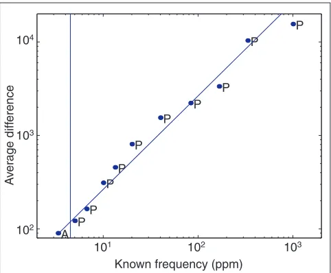
Figure 2 shows a typical plot of the spiked transcript readout from a single hybridization containing 22g of cRNA and a corresponding amount of spike-in transcripts. The specific hybridization intensity (AD) value for each of the 11 spike-in controls is plotted as a function of transcript frequency in units of transcripts per million. The points are fitted with a generalized linear model that is then used as a calibration curve to compute frequencies from the AD values of the other genes on the array. Using logistic regression, we define the chip sensitivity as the frequency where we estimate a gene to have a 70% probability of being called ‘Present’. We will use the capitalized terms ‘Absolute Decision’, ‘Present’, ‘Absent’ and ‘Marginal’ when referring to a specific value

that is calculated by the Affymetrix GeneChip software (described in Materials and methods). In Figure 2, the verti-cal line at a frequency of 4.5 indicates the computed sensitiv-ity estimate for this array.

Fitting a power law model (AD = kFn_{) to the data in Figure 2}

yields the exponent n= 0.93. This indicates mild curvature in the response, consistent with progressive saturation of array readout for the highest abundance mRNAs. Experi-ments using 0.1 to 102g cRNA per hybridization with corre-sponding amounts of spike-in transcripts, as well as high and low gain settings on the scanner, indicated that readout saturation (not hybridization saturation) accounted for most of the observed curvature in the spike-in response. The use of approximately 12g cRNA in each hybridization, or reduced scanner gain, largely eliminated saturation with no penalty in sensitivity.

Scaled frequency normalization

Frequency normalization is appealing theoretically and effec-tive even when the constant-mean assumption is known to be invalid. However, our experience suggests that frequency estimates might be biased by experimental limitations on the

Figure 2

The calibration model for frequency normalization. Eleven control transcripts are spiked into the hybridization solution at known concentrations, and the absolute difference (AD) measurements for these controls are plotted against their known frequencies. P and A represent Present and Absent calls, respectively, from Affymetrix GeneChip software. Hybridization response in average difference (AD) is approximately proportional to transcript abundance. The solid fitted line is a linear model with intercept zero, which is used to calculate frequencies for all other transcripts on the array. The vertical line at 4.5 ppm represents the calculated limit of detection for this particular array; frequencies below that level are damped to avoid attributing significance to expression differences caused by assay noise.

104

103

102

101 ₁₀2 ₁₀3

P

P

A P

P

P

P

P

P

P P

Known frequency (ppm)

A

v

er

age diff

accuracy with which control transcripts can be spiked into cRNA. Specifically, because of the combination of small fluid-handling uncertainties and potentially larger variation in the purity of cRNA preparations, the actual ratio of the spiked transcripts to cDNA-template-derived cRNAs might be significantly skewed from one array to another. One source of variable impurities in cRNA preparations could be oligo(dT)-primer-dependent cRNA product [19]. Such cRNA impurities would result in erroneous normalization in which all readouts from one array would be systematically higher or lower than those from another array. We use the term ‘spike-skew’ to denote this multiplicative skew in frequency values among multiple hybridizations. One expected symptom of spike-skew would be replicate hybridization readouts that are highly correlated but have widely divergent mean expression levels.

We developed the hybrid scaled frequency (Fs₎

normaliza-tion method to mitigate the effects of spike-skew. Fs

normal-ization is based on the principle of removing technical variation in the ratio of spiked transcripts to cDNA-template-derived cRNAs, by averaging the response to spiked cRNAs over multiple hybridizations. To compute Fs_{values, globally}

scaled average differences are first computed for all arrays in a set. This initial step implicitly makes the constant-mean assumption. A calibration function is then computed by fitting a single linear model to the scaled average differences of all spiked cRNAs on all the arrays in the dataset, pooled together. Individual array sensitivities are still computed as described above, and the same damping of low-end frequen-cies is carried out using the sensitivity values for each array.

To compare F and Fs_{metrics, consider an experimental set}

of ten arrays. To compute F values, ten linear models are fitted to the ten distinct, unscaled AD responses to the spiked cRNAs, yielding ten different calibration factors, one for each array. In contrast, when computing Fs _{values, a}

single linear model is fitted to the pooled spike response curve consisting of 10 x 11 = 121 globally scaled AD values, and a single calibration factor generated for all ten arrays. If there was no technical variation in the ratio of spiked tran-scripts to cDNA-template-derived cRNAs in the ten experi-ments, both approaches would give the same quantitation, up to a random error term arising from the difference between fitting ten 11-point responses versus a single 121-point response. If, in one of the ten arrays, the ratio of spiked transcripts to cDNA-template-derived cRNAs is dif-ferent for technical reasons, then spike response for that array will be skewed, and the F-metric readout for that array will be skewed relative to the other nine arrays. In contrast, such a skewed array will only affect the Fs _{metric to the}

extent that the single skewed response shifts the fit to the pooled spike response. The skew for the single problematic array will be removed because all arrays in the set will be scaled and calibrated with a single factor. In other words, Fs

values are estimates of transcript abundance in cRNA, based

on the average response to the spiked cRNAs over multiple hybridizations and on the sensitivity of each individual array. F values provide the same estimate, but based solely on the response to spiked cRNAs in a single array hybridization.

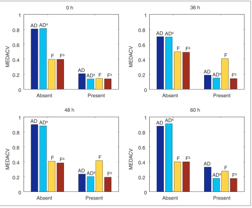
Comparison of normalization methods: reproducibility

We compared the performance of four metrics: AD; globally normalized AD (ADs_{); frequency (F); and scaled frequency}

(Fs_{). The basis for comparison was experimental data}

con-sisting of four sets of replicated hybridizations (each n= 3 or 4) of the same array design (the C. elegansA array). Perfor-mance of each metric was measured by the median absolute coefficient of variation (MEDACV) of probe sets across the replicated hybridizations. MEDACV is a measure of repro-ducibility for which a value of zero indicates perfect agree-ment of all transcript readouts in a set of replicated hybridizations. We compared MEDACV for two classes of mRNAs: those called Present in at least 50% of replicated hybridizations (referred to as ‘Present’ mRNAs), and those Present in fewer than 50% of the replicated hybridizations (referred to as ‘Absent’ mRNAs). All metrics showed higher (worse) MEDACVs for the low-abundance Absent mRNAs than for the higher-abundance Present mRNAs (Figure 3), as expected from the presence of background noise on the arrays. For Present genes, ADs_{was more reproducible than}

AD, as expected. Scaled frequency (Fs_{) was as reproducible as}

ADs_{for Present genes in all replicate sets, and yielded trivially}

higher reproducibility than ADs_{for Absent mRNAs, owing to}

damping of background noise. Frequency appeared equiva-lent to Fs_{and AD}s_{in the first set of experiments (the 0-hour}

timepoint) but had a higher MEDACV than Fs_{in the other}

three replicate sets. We also computed Pearson correlation coefficients for the same replicate readouts. Unlike MEDACV, correlation coefficients between replicate readouts were similar for all metrics (in the range from 0.978-0.996).

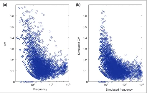
To better understand the reasons for the markedly different MEDACV performances of the four metrics on experimental replicates, we performed simulations. These simulations incorporated several adjustable noise parameters. We esti-mated values for these parameters iteratively, based on experimental data (see Materials and methods). The similar-ity in the CV distributions of experimental and simulated data indicated that, for our purposes, the simulations reca-pitulated the major error properties of real array data (Figure 4).

We tested if spike-skew could account for the relatively high CV of frequency in three of the four replicate sets (Figure 3) by comparing experimental data to simulated data with known levels of spike-skew. To approximate spike-skew, the concen-tration of the spike-in transcripts in simulations was multi-plied by a random noise term. Over a series of simulations, we varied the standard deviation of the noise term from 0 to 40% to model the effect of increasing spike-skew. MEDACV values

comment

reviews

reports

deposited research

interactions

information

were then computed from the simulation results in the same way as for the experimental data in Figure 3.

As expected, only frequency was sensitive to spike-skew (Figure 5). The Fs_{metric, which uses a single standard curve}

pooled from each dataset to normalize all arrays in that dataset, effectively eliminated spike-skew effects. In the sim-ulations, a spike-skew level of 20% led to MEDACV values for frequency in simulated replicates that were much higher than those of ADs _{or F}s_{. These results were highly}

reminis-cent of the 36, 48 and 60 hour experimental replicate sets (compare Figures 5 and 3).

Taken together, the experimental data and the simulations suggest that spike-skews of roughly 20% can explain the sometimes inferior MEDACV (but consistently high inter-replicate correlation coefficients) of the frequency metric.

Comparisons across array designs

We next considered the reproducibility of readouts of the same mRNA on different array designs. For this analysis, we selected the three mRNAs that were monitored by identical probe sets on each of the A, B, and C array designs and were called Present in all hybridizations of the 0 hour cRNA sample. The observed CV of the ADs_{metric was in all cases}

Figure 3

Reproducibility of four normalization methods. For each of four developmental stages in a C. elegansdata set (0, 36, 48 and 60 h, see [10]), the figure shows the median absolute coefficient of variation (MEDACV) for each normalization method, for genes that are primarily Absent or primarily Present in replicate hybridizations. For Absent genes, frequency methods have lower MEDACV than AD methods because of the damping of low-end noise. For Present genes, Fs_{and AD}s_{are roughly}

equivalent and outperform the unscaled methods in all cases. Numbers of replicate hybridizations were three (36 h sample) or four (0, 48, 60 h samples).

Absent

Present

0

0.2

0.4

0.6

0.8

1

AD AD

F

F

AD

AD

_F

_F

0 h

MED

A

CV

Absent

Present

0

0.2

0.4

0.6

0.8

1

AD AD

F

F

AD

AD

F

F

36 h

MED

A

CV

Absent

Present

0

0.2

0.4

0.6

0.8

1

AD AD

F

_F

AD

_AD

F

F

48 h

MED

A

CV

Absent

Present

0

0.2

0.4

0.6

0.8

1

AD

AD

F

F

AD

AD

F

F

60 h

MED

A

larger than that of the F or Fs_{metric, and was greater than}

0.55 for all three mRNAs, indicating very poor agreement of readouts from different array designs when global normal-ization was used (Figure 6). In contrast, the CVs of both F and Fs_{metrics were lower, with CVs for F}s_{in particular}

aver-aging 0.19 (range 0.13-0.29). The mRNA K11C4.5 was expressed at > 10-fold lower levels than either of the other two mRNAs, and thus had higher CV values for both F and Fs _{than the other two mRNAs. Comparison of the across}

-array-design CVs to the within-array-design CVs for the three transcripts in Figure 6 indicates that the reproducibil-ity of ADs_{was substantially poorer when comparing across}

array designs rather than within arrays. Specifically, ADs

across-array CV was 3.2- to 6.4-fold higher than the within-array CV. In contrast, the across-within-array CV for Fs _{was only}

1.3- to 1.6-fold higher than the corresponding within-array CV (Table 2).

The reason for the poor agreement of ADs_{readouts across}

distinct designs was that the mRNAs monitored by the A array are, on average, expressed at higher levels than those on the B or C array, as confirmed by two independent lines

of evidence. First, the mRNAs on the A array were inten-tionally selected because they were represented in

C. elegans cDNA libraries, whereas the B and C array

genes (many of them computational predictions) were generally not represented in cDNA libraries. Second, A array mRNAs were more likely than B or C array mRNAs to be detected in the developmental time course by the Affymetrix Absolute Decision metric [10]. Because of this systematic difference between gene sets, the mean AD of all A array genes was substantially higher than that of the genes on the B or C arrays. The ADs _{metric scales data}

under the assumption that mean expression levels for all arrays should be equal. Therefore, ADs_{values for genes on}

the B and C arrays were inappropriately inflated relative to ADs_{values from the A array.}

Comparison of normalization methods: accuracy

Normalization methods should accurately measure true bio-logical variation. We tested the accuracy of the four methods using simulated data. As a baseline we chose the experimen-tal data from one of the 0-hour replicates on the A array. We generated 19 simulated experimental conditions to produce

comment

reviews

reports

deposited research

interactions

information

refereed research

Figure 4

Noise distributions (CV) for the experimental and simulated data sets. (a) 0-hour dataset; (b) simulated dataset. Simulation noise parameters were iteratively estimated from the real data (see Materials and methods). The resulting distributions were sufficiently similar to allow the use of simulations to explore the effects of different sorts of noise on normalization methods.

10

₁₀

₁₀

₁₀

₁₀

₁₀

0

0.1

0.2

0.3

0.4

0.5

0.6

Frequency

CV

0

0.1

0.2

0.3

0.4

0.5

0.6

Simulated frequency

Sim

ulated CV

20 raw average difference values for each of 6,617 genes. For each of the four metrics, computed fold-changes between the modulated condition and the baseline (considering only messages called Present) were compared to the true fold-changes. Accuracy was defined as the fraction of computed fold-changes that were accurate within twofold, and deter-mined for assumed levels of spike-skew from 10-40% (per-centage is the ratio of standard deviation (SD) to mean of the random spike-skew term in the simulation). Three simula-tions were carried out at each level of assumed spike-skew. ADs_{and F}s_{metrics performed equally well and best overall,}

with accuracies above 99% regardless of spike-skew. As expected, frequency was the only metric with a significant

dependence on the level of spike-skew. At 10% spike-skew, frequency accuracy was (mean H SD) 0.9951H0.0006, at 20%, 0.96_H0.02, and at 40%, 0.82_H0.06. For comparison, the accuracy of AD was 0.88H0.07 at 10% spike-skew, and did not change significantly at higher spike-skew levels.

We stress that the overall accuracy levels reported here are highly dependent on adjustable parameters in our simula-tion model (see Materials and methods). Nevertheless, the simulations demonstrate that at levels of spike-skew consis-tent with our experience, scaled frequency is as accurate as globally normalized ADs_{; this observation is robust to}

changes in the model parameters.

Figure 5

Reproducibility of normalization methods for different degrees of spike-skew in simulated data. The SD of the random multiplicative spike-skew term in the simulations was adjusted from 0.1 to 0.4 (10-40%). Increasing spike-skew specifically degrades the performance of the F metric. Note that the relatively poor performance of F relative to Fs_{and AD}s_{when the}

spike-skew is 0.2 (20%) is similar to that observed in the experimental data (Figure 3). Twenty simulated hybridizations were generated for each level of spike-skew.

Absent

Present

0

0.2

0.4

0.6

0.8

1

AD

AD

s

F

F

_AD

AD

_F

_F

Spike-skew SD = 0.000000

MED

A

CV

Absent

Present

0

0.2

0.4

0.6

0.8

1

AD

AD

s

F

F

AD

AD

F

_F

Spike-skew SD = 0.100000

Spike-skew SD = 0.400000

Spike-skew SD = 0.200000

MED

A

CV

Absent

Present

0

0.2

0.4

0.6

0.8

1

AD

AD

F

F

AD

AD

F

F

MED

A

CV

Absent

Present

0

0.2

0.4

0.6

0.8

1

AD

AD

F

F

AD

AD

F

F

MED

A

Absolute quantitation of cRNA and cellular RNA

There are several potential sources of inaccuracy in the cRNA quantitiation given by the scaled frequency metric.

Our results suggest that there is significant uncertainty in the molar ratio of spike-in mRNAs to template-derived cRNAs in any hybridization (the spike-skew effect). The MEDACV for the F metric in Figure 3 is likely one measure of this uncertainty, as it probably arises primarily from cRNA purity variation. This uncertainty leads to propor-tional differences between frequency metric readouts and true cRNA transcript abundances. However, in the scaled frequency method, the simultaneous normalization of larger datasets reduces these differences through averaging. We anticipate that inaccuracies of cRNA quantitation arising from this effect will be reduced by improved methods for quantitation of cRNA preparations.

For F and Fs_{, heterogeneity in probe response will lead to}

gene-specific biases in quantitation. Our data contains two observations that allow us to estimate the degree of hetero-geneity among spiked probe sets. Cursory examination of the calibration curve (Figure 2) suggests relative responses of the 11 distinct probe sets shown do not vary more than two-fold: no observations fall more than about a factor of two from the fitted line. A more rigorous evaluation of probe set hetero-geneity can be done by comparing the ratio of AD values from two distinct probe sets that monitor the same transcript in a single hybridization. This ratio estimates the difference in readout that would be observed for a single transcript if a dif-ferent probe set were selected. This comparison was made for the 11 spiked transcripts (each array contained two probe sets for each of these mRNAs). On the basis of 138 ratio measure-ments from the C. elegansarrays, the 10th-90th percentile range for the ratio was 0.39-1.44 [10], indicating that for the

comment

reviews

reports

deposited research

interactions

information

refereed research

Figure 6

Reproducibility of comparisons across array designs. The CV of repeated measurements of three genes across three array designs is shown for the four metrics. Frequency (F) and scaled frequency (Fs_{) were more reproducible than either average}

difference (AD) or scaled average difference (ADs_).

K10B3.8

K11C4.5

M03F4.2

0

0.1

0.2

0.3

0.4

0.5

0.6

0.7

0.8

0.9

1

AD

AD

F

F

AD

AD

F

F

AD

AD

F

F

0 h

CV across three arr

a

set of control transcripts, the uncertainty in cRNA quantita-tion due to heterogeneity in probe set responses for 80% of transcripts was less than threefold.

In addition to these factors leading to inaccuracies in cRNA quantitation, there are at least two important factors leading to differences between cRNA abundances and cellular RNA abundances in the starting biological material.

First, because cRNA is generated from the polyadenylated fraction of total cellular RNA by a linear amplification process, frequency estimates will not reflect sample-specific changes in the fraction of polyadenylated RNA in total cellu-lar RNA. This may be a desirable feature of frequency esti-mates, in cases where per-total-RNA abundance is less relevant than per-polyadenylated-RNA abundance.

Second, any gene-specific biases in the cRNA amplification procedure will lead to gene-specific differences between cRNA and per-total-RNA quantifications. Evidence to date suggests that these biases are small [1] and reproducible [19].

Taken together, the above-noted sources of inaccuracy suggest that there can typically be around two- to threefold differences between scaled frequency per-cRNA estimates and per-polyadenylated-RNA abundances in the starting material. These differences could be reduced by improved cRNA process control and quantitation, and by improved probe selection algorithms.

Conclusions

We have shown that cRNAs spiked into hybridization solu-tions at known concentrasolu-tions covering two to three orders of magnitude can be used to normalize array data and to

estimate array sensitivity. However, frequency normaliza-tion based solely on these control transcripts can be adversely affected by variations in the ‘purity’ of cRNA preparations. These observations underline the need for meticulous quality control during the production of cRNA samples and accurate quantitation of the resulting material. With better control of these processes, the frequency metric may provide a robust spike-based normalization that, unlike all the other metrics described here, does not rely on the constant-mean assumption.

In the presence of variation in cRNA purity, the Fs _metric

provides a compromise between the robustness of the ADs

metric and the more absolute quantitation scale of the fre-quency metric, in cases where the constant-mean assump-tion is valid. In addiassump-tion, the Fs_{metric provides a common}

scale for comparing data from distinct array designs. This is an important advantage over other metrics. For example, the Fs _{metric allows comparison of the expression levels of all}

worm mRNAs on all three of our array designs with compa-rable confidence to within-array-design comparisons. This is not possible with globally normalized average differences. We believe that cRNA quantitation and the damping of low-amplitude signals provided by the Fs _{normalization make}

this metric a valuable format for reporting diverse gene expression array results.

Materials and methods

Array experiments used the Genetics Institute C. elegans

Affymetrix GeneChip_oligonucleotide arrays, a set of three arrays (denoted A, B and C) which in aggregate monitor approximately 98% of the 19,099 predicted worm mRNAs in the October 1998 worm genome sequence release [20]. The total number of probe sets on each array was 6,617 (A array), 5,768 (B), and 6,646 (C). Each probe set consists of 20 dis-tinct probe pairs (each probe is a 25mer) designed to monitor a single transcript. On the C. elegans arrays described here, probe sets monitoring the spiked transcripts were each tiled twice with a different set of oligonucleotide probes. On arrays that are commercially available from Affymetrix, one probe set is tiled to monitor each of the spike-in transcripts. The probe sets are not fully randomly distributed across the arrays, although on the C. elegans

arrays the different probe sets are tiled in widely different regions of the arrays. Experimental array data described here were taken from the developmental time course dataset reported in [10]. Specifically, we examined individual repli-cate hybridizations of the A array from the worm develop-mental time course at each of 0 (n= 4), 36 (n= 3), 48 (n= 4) and 60 (n= 4) hours after synchronization of worm eggs by bleach, as well as a larger set of 13 hybridizations of all three arrays to samples ranging from oocytes to 2-week-old worms. Replicate hybridizations in the datasets included independently generated complementary RNA (cRNA)

Table 2

Ratios of across- to within-array coefficients of variation (CVs)

Metric Transcript

K10B3.8 K11C4.5 M03F4.2

AD 2.9 4.2 3.6

ADs _{6.4 3.2 6.1}

F 2.8 3.0 2.7

Fs _{1.3 1.6 1.5}

preparations from the same starting total RNA. Primary data for all transcripts on all arrays (including all replicates of all three array designs) is contained in the supplementary Excel spreadsheet (see Additional data files).

Spike-in transcript pool

A pool of biotin-labeled spike-in control transcripts was derived by in vitrotranscription of 11 cloned Bacillus subtilis

genes, using the methods described in [21]. The spike-in pool was added into hybridization cocktails in proportion to the UV-quantitated cRNA mass in the hybridization, so as to achieve the desired final concentration of spike-ins. The spiked transcripts and their final concentrations in the hybridization cocktails are listed in Table 1. Final concentra-tions in pmol and parts per million (ppm) for each spiked transcript were computed from the known length of each spike-in, assuming a total mass of 2 ₂g worm cRNA in a 2002l hybridization volume, and an average length of 1,000 bases for in vitrotranscribed worm cRNAs.

Metrics for transcript abundance

Average difference (AD) is the basic measure of transcript abundance that is calculated by the Affymetrix GeneChip 3.1 software. The calculation of AD is described in detail in the Affymetrix GeneChip User Guide [17]. Briefly, a background intensity is computed for each of 16 rectangular sectors on the array. This local background is subtracted from the intensity values of each probe cell in all sectors. After back-ground subtraction, the difference between perfect match (PM) and mismatch (MM) feature intensity is calculated for all probe pairs in each probe set (in our case, 20 probe pairs in total). The AD for each probe set is the average of the PM -MM differences, after outlying values are removed.

A second important metric generated by the GeneChip soft-ware is the Absolute Decision. The Absolute Decision is a categorical call for each transcript: either Present, Absent, or Marginal. The Absolute Decision is a heuristic metric based on the number of probe pairs for a given transcript that show strong specific hybridization signals. See the Affymetrix GeneChip User Guide [17] for a detailed descrip-tion of this metric.

Because of array-to-array variation in overall signal strength, AD values from different arrays are usually normalized to a common scale. We reproduced the scaled AD normalization of the Affymetrix GeneChip 3.1 software. The calculation is described in detail in the Affymetrix GeneChip User Guide [17]. Scaling is done by equalizing the average intensity of all arrays in a given dataset, where the average intensity is defined as the trimmed average of the AD values of every probe set on the array, excluding the highest 2% and lowest 2% of the values. This normalization works on the assumption that the summed expression level of all genes on the array is constant across experiments, and that differences in expres-sion levels between arrays can be corrected by array-specific

scaling factors. We denote the normalized AD values as scaled average difference (ADs_).

The calculation of frequency (F) values involved two steps: first, conversion of AD values to frequencies by use of the calibration curve, and second, estimation of the chip sensi-tivity of detection and ‘damping’ of frequency values below this sensitivity.

The calibration curve for each hybridization was constructed from the AD values for each of the 11 control transcripts and their known frequencies (Table 1). AD values that were nega-tive, or associated with Absent or Marginal Absolute Deci-sions, were removed from the curve in order to improve the robustness of the fit. This calibration curve was fitted by a linear function with zero intercept, using a generalized linear model [22] fitting procedure in the statistical software S-PLUS (Insightful Corp., Seattle, WA). The fitting proce-dure assumed a gamma error structure, appropriate for data with constant coefficient of variation, and utilized iterative reweighting of errors. The single coefficient of this linear fit was multiplied with the average difference values for each gene on the array to yield initial frequency estimates. Cali-bration curves for the hybridizations described here were examined visually to rule out poor curve fits.

Chip sensitivity of detection was estimated from the Absolute Decisions (Present, Marginal, or Absent) for the 11 spike-in transcripts in one of two ways. In the general case, Absolute Decisions were considered as a binary response: Absent = 0, Present = 1, with Marginal calls treated as Absent to be conservative. This response was regressed against the log-transformed known frequencies, using a gen-eralized linear model with a logit link function. The chip sen-sitivity was then defined as the frequency at which the predicted odds of a Present call were 70%. In the special case where all spike-in mRNAs called Absent were lower-abun-dance messages than all spike-ins called Present, the sensi-tivity was defined by linear interpolation as the frequency 70% of the distance between the highest Absent call fre-quency and the lowest Present call frefre-quency.

Frequency values for all genes on the array that fell below the sensitivity were damped as follows. Negative frequencies (corresponding to negative AD values) were adjusted to one-half of the chip sensitivity. Frequencies between zero and the chip sensitivity were adjusted to the average of the frequency and the chip sensitivity. The rationale for this adjustment was threefold. First, one-half the chip sensitivity was a rea-sonable a prioriestimate of abundance for many genes that were not reliably detected. Second, the adjusted frequencies were guaranteed to be positive-valued, making downstream analyses of frequency values (for example, log transforma-tion) significantly easier. Third, retaining the adjusted low-level frequency estimates was preferable to discarding them, because discarding the values would make it impossible to

comment

reviews

reports

deposited research

interactions

information

detect potentially important regulation of these genes in future experiments.

Frequency normalization could be adversely affected by technical uncertainties in cRNA preparation (see Results and discussion). To attenuate these effects, an additional fre-quency variant termed scaled frefre-quency (Fs_{) was introduced.}

Fs_{was a hybrid of ADs and frequency, and was computed as}

follows. ADs _{was first computed for a set of two or more}

arrays exactly as described above. Then a linear model (with zero intercept) was fitted to the pooled ADs_{values for the 11}

spike-in transcripts from all arrays, ignoring negative ADs

values or those associated with Marginal/Absent Absolute Decisions. The slope of this linear model was the single cali-bration factor for the entire dataset. This slope was multi-plied with the ADs_{values from all arrays to yield F}s_values.

Per-array sensitivity values were computed exactly as described for F, and Fs_{values on any array that were below}

the array sensitivity were adjusted as described above.

Simulated data

Array data was simulated as follows. First, a single experi-mental dataset, one of the 0-hour replicates, was chosen as a baseline for generation of all simulated data. To this baseline dataset, several random noise sources were added to repro-duce key sources of variability in array data. The relation describing the simulated data was:

AD_ij= b_ij+ ADB_i (a_j m_ij s_ij r_ij)

where

AD_ij= simulated AD for the ith mRNA on the jth array

ADB_i= baseline gene expression data for the ith mRNA

b_ij= background noise for the ith mRNA on the jth array

a_j= array intensity offset for the jth array

m_ij= multiplicative noise for the ith mRNA on the jth array

s_ij= spike-skew factor for the ith mRNA on the jth array (unity for all nonspiked mRNAs)

r_ij= regulation factor for the ith gene on the jth array (unity for all spiked mRNAs)

Background b_ijwas Gaussian with a standard deviation (SD) that varied randomly from one array to another. The back-ground noise SD had a mean of 20 AD units, and a standard deviation of 5 AD units. Array intensity offsets a_j were Gaussian with a mean of one and SD of 0.3. Multiplicative noise, m_ij, was drawn from a normally distributed zero-mean noise source with a constant CV of 0.1. Spike-skew factor s_ij

was a single random factor for all spiked cRNAs on a given

array, and unity for all other messages. The spike-skew factor for the spiked cRNAs was Gaussian with mean 1 and a SD that was adjusted from 0.1 to 0.4 (in percentage terms, 10-40%). Regulation factors r_ijwere generated by a proce-dure in which the base-10 log (fold-change) for each gene was selected from a normal distribution with mean 0 and SD 0.5. Extreme random regulation factors were limited so that the regulated gene expression values had the same range as baseline data. After multiplication of each gene by its regula-tion factor, the mean expression level of all genes was adjusted so that the overall mean expression level was unchanged by regulation.

Additional data files

Primary data for all experimental hybridizations are pro-vided with the online version of this article.

Acknowledgements

We thank Yizheng Li, Bill Mounts and Scott Jelinsky for thought-provoking conversations about normalization approaches, Steve Rozen and Ken Grif-fiths for related software and database implementations, and Michael Byrne for contributions to initial normalization concepts.

References

1. Lockhart DJ, Dong H, Byrne MC, Follettie MT, Gallo MV, Chee MS, Mittmann M, Wang C, Kobayashi M, Horton H, Brown EL: Expres-sion monitoring by hybridization to high-density oligonu-cleotide arrays.Nat Biotechnol1996, 14:1675-1680.

2. Affymetrix: Affymetrix GeneChip Expression Analysis Technical Manual. Santa Clara: Affymetrix; 2000.

3. Harkin DP, Bean JM, Miklos D, Song YH, Truong VB, Englert C, Chris-tians FC, Ellisen LW, Maheswaran S, Oliner JD, Haber DA: Induction of GADD45 and JNK/SAPK-dependent apoptosis following inducible expression of BRCA1.Cell1999, 97:575-586.

4. Wodicka L, Dong H, Mittmann M, Ho MH, Lockhart DJ: Genome-wide expression monitoring in Saccharomyces cerevisiae.Nat Biotechnol 1997, 15:1359-1367.

5. Alon U, Barkai N, Notterman DA, Gish K, Ybarra S, Mack D, Levine AJ: Broad patterns of gene expression revealed by clustering analysis of tumor and normal colon tissues probed by oligonucleotide arrays. Proc Natl Acad Sci USA1999, 96:6745-6750.

6. Selinger DW, Cheung KJ, Mei R, Johansson EM, Richmond CS, Blat-tner FR, Lockhart DJ, Church GM: RNA expression analysis using a 30-base pair resolution Escherichia coli genome array.Nat Biotechnol2000, 18:1262-1268.

7. Cho RJ, Campbell MJ, Winzeler EA, Steinmetz L, Conway A, Wodicka L, Wolfsberg TG, Gabrielian AE, Landsman D, Lockhart DJ, Davis RW: A genome-wide transcriptional analysis of the mitotic cell cycle.Mol Cell1998, 2:65-73.

8. Schuchhardt J, Beule D, Malik A, Wolski E, Eickhoff H, Lehrach H, Herzel H: Normalization strategies for cDNA microarrays. Nucleic Acids Res 2000, 28:e47.

9. Hartemink AJ, Gifford DK, Jaakkola TS, Young RA: Maximum like-lihood estimation of optimal scaling factors for expression array normalization. Available at [http://www.psrg.lcs.mit.edu/ publications/Papers/spie.pdf]

10. Hill AA, Hunter CP, Tsung BT, Tucker-Kellogg G, Brown EL: Genomic analysis of gene expression in C. elegans. Science 2000, 290:809-812.

11. Holstege FCP, Jennings EG, Wyrick JJ, Lee TI, Hengartner CJ, Green MR, Golub TR, Lander ES, Young RA: Dissecting the regulatory circuitry of a eukaryotic genome.Cell1998, 95:717-728. 12. Yang YH, Dudoit S, Luu P, Speed TP: Normalization for cDNA

Microarray Data.Available at

13. Li C, Wong WH: Model-based analysis of oligonucleotide arrays: Expression index computation and outlier detection. Proc Natl Acad Sci USA2001, 98:31-36.

14. Schadt EE, Li C, Su C, Wong WH: Analyzing high-density oligonucleotide gene expression array data. J Cell Biochem 2000, 80:192-202.

15. Kepler T: Normalization and Statistics for Microarray Data by Self-Consis-tency and Local Regression. Available at [http://www.ipam.ucla.edu/ publications/fg2000/fgsn_tkepler.ppt]

16. Lee CK, Klopp RG, Weindruch R, Prolla TA: Gene expression profile of aging and its retardation by caloric restriction. Science1999, 285:1390-1393.

17. Affymetrix: GeneChip Analysis Suite User Guide (Version 3.3). Santa Clara: Affymetrix; 1999.

18. Ishii M, Hashimoto S, Tsutsumi S, Wada Y, Matsushima K, Kodama T, Aburatani H: Direct comparison of GeneChip and SAGE on the quantitative accuracy in transcript profiling analysis. Genomics2000, 68:136-143.

19. Baugh LR, Hill AA, Brown EL, Hunter CP: Quantitative analysis of mRNA amplification by in vitrotranscription.Nucleic Acids Res 2001, 29:e29.

20. The C. elegansSequencing Consortium: Genome sequence of the nematode C. elegans: a platform for investigating biology. Science1998, 282:2012-2018.

21. Byrne MC, Whitley MZ, Follettie MT: Preparation of mRNA for expression monitoring. In Current Prototcols in Molecular Biology. New York: John Wiley & Sons; 2000:22.2.1 - 22.2.13.

22. McCullagh P, Nelder JA: Generalized Linear Models. Cambridge: Cam-bridge University Press; 1989.

comment

reviews

reports

deposited research

interactions

information