Study of the Fastest Rate of Freezing Saline Solution
Using Factorial Design Method
Nia Nuraeni Suryaman
Department of Mechanical Engineering, Widyatama University, Indonesia
Copyright©2019 by authors, all rights reserved. Authors agree that this article remains permanently open access under the terms of the Creative Commons Attribution License 4.0 International License
Abstract An engineer needed the ability to design an
experiment research to be effective and efficient to obtain optimal results. The purpose of this experiment is to determine the fastest rate of freezing saline solution. The research process begins with determining the independent variables as much as possible and determines the three independent variables to be tested. After determine variables, and then create table factorial design to determine the research steps as much as 8 times. Then determine the most influential variables using Yates's algorithm was then tested again using response surface methodology (RSM), but for this study only uses two steps of the three step RSM. So it can be concluded that the lower temperature and salinity the faster the rate of freezing for both type of salt, Krosok and salt.Keywords Rate of Freezing, Saline Solution, Factorial
Design1. Introduction
An engineer needed the ability to design an experiment research to be effective and efficient to obtain optimal result. These experiments use factorial design methods to make it easier for researchers to get effective and efficient results.
Factorial design is a method for determining the influence of several independent variables on the response. Basically an experiment is designed to determine one variable in one response. Therefore, factorial design can make it easier to experiment with more than one
independent variable. Another use of factorial design is that it can reduce the number of experiments we have to do by studying several factors simultaneously.
The purpose of this experiment is to determine the fastest rate of freezing saline solution. The output to be produce of this study is a graph and the most influential variable as a result. In this study the output will be obtained by using factorial design and least square and response surface methodology.
2. Literature Study
2.1. Factorial Design
Factorial design is an important method to determine the effects of multiple variables on a response/output.
Traditionally, experiments are designed to determine the effect of one variable upon one response/output.
There are advantages by combining the study of multiple variables in the same factorial experiment. Factorial design can reduce the number of experiments one has to perform by studying multiple factors simultaneously. Additionally, it can be used to find both main effects (from each independent factor) and interaction effects (when both factors must be used to explain the outcome).
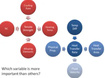
Figure 1. Important Variable
2.2. Least Square
The method of least squares is a standard approach to the approximate solution of over determined systems, i.e., sets of equations in which there are more equations than unknowns.
Least square means that the overall solution minimizes the sum of the squares of the errors made in the results of every single equation. The most important application is in data fitting.
In this equation the β's are unknown constants to be estimated and the x have known values. One common example is where x1, x2,... are the levels of k factors, say temperature x1, line speed x2, concentration x3, and so on, and y is a measured response such as yield.
0 0 1 1 2 2 k k
y= βx + βx + βx + + β... x +e
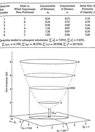
Table 1 shows a small illustrative set of data from an experiment to determine how the initial rate of formation of an undesirable impurity y depended on two factors: A) the concentration xo of monomer and B) the concentration of
dimer x1. The mean rate of formation y was zero when both components x0 and x1 were zero. Over the relevant ranges of x0 and x1 the relationship was expected to be approximated by
0 0 1 1
y= βx + βx +e
For any particular set of trial values of the parameters 𝛽0 and 𝛽1 could calculate S(𝛽). For example, for data of Table 1, if 𝛽0= 1 and 𝛽1= 7, would get:
𝑆(1,7) =�(𝑦 −1𝑥0−7𝑥1)2= 1.9022
Thus in principle could obtain the minimum value of S by repeated calculation for a grid of trial values. It would eventually be able to construct Figure 2, a 3D plot of the sum of squares surface of S(𝛽) versus 𝛽0 and 𝛽1. The coordinates of the minimum value of this surface are the desired least square estimates
Table 1. Initial Rate of Impurity Investigation
Figure 2. Sum of Square Surface: 𝑆(𝛽) =∑(𝑦 − 𝛽0𝑥0− 𝛽1𝑥1)2
2.3. Normal Equation
( )
(
)
( )
(
)
0 0 0 1 0
0
0 0 0 1 1
1 S
2 y x x x 0
S
2 y x x x 0
∂ β
= − Σ − β − β = ∂β
∂ β
= − Σ − β − β = ∂β
After simplification these become what are called the normal equations
2
0 0 1 0 1 0
2
0 0 1 1 1 1
b
x
b x x
yx
b
x x
b x
yx
Σ + Σ
= Σ
Σ
+ Σ = Σ
3. Research Methodology
1) Determined Independent Variable
The independent variables determined for the design of this experiment are as follows:
a) Freezer Temperature b) Refrigerator
c) Salinity
d) Frozen water mass e) Freezing time
f) Initial water temperature g) Type of water
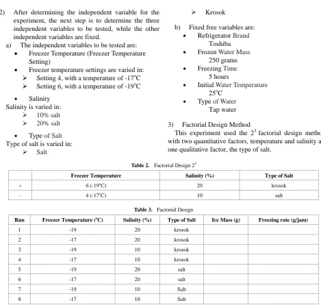
[image:3.595.131.463.88.546.2]2) After determining the independent variable for the experiment, the next step is to determine the three independent variables to be tested, while the other independent variables are fixed.
a) The independent variables to be tested are: • Freezer Temperature (Freezer Temperature
Setting)
• Freezer temperature settings are varied in:
Setting 4, with a temperature of -17oC
Setting 6, with a temperature of -19oC • Salinity
Salinity is varied in:
10% salt
20% salt
• Type of Salt
Type of salt is varied in:
Salt
Krosok
b) Fixed free variables are: • Refrigerator Brand
Toshiba • Frozen Water Mass
250 grams • Freezing Time
5 hours
• Initial Water Temperature
25oC • Type of Water
Tap water 3) Factorial Design Method
This experiment used the 23 factorial design methods with two quantitative factors, temperature and salinity and one qualitative factor, the type of salt.
Table 2. Factorial Design 23
Freezer Temperature Salinity (%) Type of Salt
+ 6 (-19oC) 20 krosok
[image:4.595.58.528.68.513.2]- 4 (-17oC) 10 salt
Table 3. Factorial Design
Run Freezer Temperature (oC) Salinity (%) Type of Salt Ice Mass (g) Freezing rate (g/jam)
1 -19 20 krosok
2 -17 20 krosok
3 -19 10 krosok
4 -17 10 krosok
5 -19 20 salt
6 -17 20 salt
7 -19 10 Salt
8 -17 10 Salt
4. Results and Discussion
1) The experiment was carried out in 8x according to the design factorial table that was made before. Table 4. Experiment Result
Freezer Temperature (◦C) Salinity (%) Type of Salt Ice Mass (g) Freezing Rate (g/jam)
-19 20 Krosok 30 6
-17 20 Krosok 0 0
-19 10 Krosok 210 42
-17 10 Krosok 150 30
-19 20 Salt 0 0
-17 20 Salt 0 0
-19 10 salt 160 32
-17 10 salt 170 34
2) The Most Influential Variables
[image:4.595.312.447.77.241.2] [image:4.595.70.525.299.514.2]Table 5. Yates Algorithm
Freezing Rate (g/jam) Yates Algorithm
1 2 3 divider explanation
6 6 78 144 8 18 average
0 72 66 -16 4 -4 Freezer Temperature
42 0 -18 132 4 33 Salinity
30 66 2 -4 4 -1 Setting & Salinity
0 -6 66 -12 4 -3 Salinity
0 -12 66 20 4 5 Type & Temperature
32 0 -6 0 4 0 Type & Salinity
34 2 2 8 4 2 Type, Temperature & Salinity
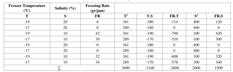
Yates algorithms table above shows that the most influential variable is the salinity. 3) Result of Least Square Method
Table 6. Least Square
Freezer Temperature
(oC) Salinity (%)
Freezing Rate (gr/jam)
T S FR T2 T.S FR.T S2 FR.S
-19 20 6 361 -380 -114 400 120
-17 20 0 289 -340 0 400 0
-19 10 42 361 -190 -798 100 420
-17 10 30 289 -170 -510 100 300
-19 20 0 361 -380 0 400 0
-17 20 0 289 -340 0 400 0
-19 10 32 361 -190 -608 100 320
-17 10 34 289 -170 -578 100 340
∑ 2600 -2160 -2608 2000 1500
Normal Equation:
b0∑T2
+ b1∑TS= FRT b0∑TS + b1∑S2 = FRS From the least square table, the normal equation becomes:
2600 b0 - 2160 b1 = -2608 -2160 b0 + 2000 b1 = 1500 To find the value of b0 and b1 use the Matrix, so that it is obtained: b0 = -3.6976
b1 = -3.24341
So the equation obtained is: FR = - 3.697 T - 3.243 S
4) Response Surface Methodology (RSM) a) Krosok
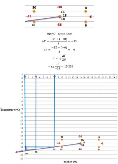
The first step is to use the initial first order method. This step takes 7 times experiments. Table 7. Krosok Initial First Order Results
No Salinity (%) Temperature ( o
C) Ice Mass (gram) Freezing Rate (g/hour)
1 20 -19 30 6
2 20 -17 0 0
3 10 -19 210 42
4 10 -17 150 30
5 15 -18 80 16
6 15 -18 90 18
[image:5.595.67.527.90.210.2] [image:5.595.63.529.262.407.2]Determination of angles used using calculations:
Figure 3. Krosok Angle
∆𝑋=−36 + (2−30)=−33
∆𝑌=−12 + (2 −6)=−9
𝛼=𝑡𝑔∆𝑋∆𝑌
=𝑡𝑔−−33 = 15.2559
Figure 4. Graph of Experimental Results in Krosok
b) Salt
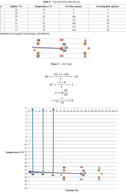
[image:6.595.102.491.98.637.2]Table 8. Salt Initial First Order Result
No Salinity (%) Temperature ( o
C) Ice Mass (gram) Freezing Rate (g/hour)
1 20 -19 0 0
2 20 -17 0 0
3 10 -19 160 32
4 10 -17 170 34
5 15 -18 100 20
6 15 -18 110 22
7 15 -18 100 20
Determination of angels used using calculation:
Figure 5. Salt Angle
∆𝑋=−32 + (2−34)=−33
∆𝑌=−2 + 02 =−1
𝛼=𝑡𝑔∆𝑋∆𝑌
=𝑡𝑔−−33 = 1.741
[image:7.595.86.520.77.743.2]5. Conclusions
In both types of salt cannot carry out RSM experiments for the first order secondary steps. This is caused by the following [3, 4, 5]:
a. The results show that the value continues to decrease with a maximum freezing rate of 50 g/hour and constant for Krosok and 48 g/hour and continues to decrease to 50 g/hour constant for salt.
b. Change in the percentage of salinity is limited because if the water adds more salt, it will become saturated so that it cannot dissolve completely. c. The freezer temperature changes are limited
according to the specifications of the refrigerator. On the graph of the Krosok, the freezing rate tends to the bottom left at an angle of 15.25o. On the graph of the salt, the freezing rate tends to the upper left with an angle of 1.74o. This indicates that the salinity is more influential than the temperature of the freezer.
The results obtained for both types of salt are, the lower the salt content, the faster the freezing rate. As for the type of salt, the fastest freezing rate according to the results of the data obtained is salt.
REFERENCES
[1] Oehlert, Gary W, (2010), “A First Course in Design and Analysis of Experiments”.
[2] P. Beckel, P. Diggle, (1999), “Linear Models Least Square and Alternative”, Second Edition, Springer.
[3] Jabarullah, N.H. (2019) Production of olefins from syngas over Al2O3 supported Ni and Cu nano-catalysts, Petroleum Science and Technology, 37 (4), 382 – 385.
[4] Jabarullah, N.H. & Othman, R. (2019) Steam reforming of shale gas over Al2O3 supported Ni-Cu nano-catalysts, Petroleum Science and Technology, 37 (4), 386 – 389. [5] Singh, A. K., & Issac, J. (2018). Impact of Climatic and
Non-climatic Factors on Sustainable Livelihood Security in Gujarat State of India: A Statistical Exploration. Agriculture and Food Sciences Research, 5(1), 30-46.