NOR AKMAL BINTI ALIAS
A project report submitted in partial fulfillment of the requirement for the award of the degree
Master of Electrical Engineering
Faculty of Electrical and Electronic Engineering University Tun Hussein Onn Malaysia
v
ABSTRACT
ABSTRAK
vii
TABLE OF CONTENTS
TITLE i
DECLARATION ii
DEDICATION iii
ACKNOWLEDGEMENT iv
ABSTRACT v
TABLE OF CONTENTS vii
LIST OF TABLES xi
LIST OF FIGURE xii
LIST OF SYMBOLS AND ABBREVIATION xv
LIST OF APPENDICES xvi
CHAPTER 1 INTRODUCTION
1.1 Project Background 1
1.2 Problem Statements 2
1.3 Project Objectives 2
1.4 Project Scopes 2
CHAPTER 2 LITERATURE REVIEW
2.1 PID Controller 4
2.2 2.3
LQR Controller Inverted Pendulum
2.3.1 Rotary Position Sensor
2.3.2 Motor with encoder (SPG30-20K)
2.4
2.5 2.6
2.3.2 Motor Driver L293 MATLAB
2.4.1 MATLAB Simulink 2.4.2 M-File
Arduino MEGA 2560
Inverted Pendulum Example in Real Life and Previous Case Study
2.6.1 Inverted Pendulum Example in Real Life 2.6.2 Previous Case Study
2.6.2. 1 LQG/LTR Controller Design for Rotary Inverted Pendulum Quanser Real-Time Experiment
2.6.2.2 DC Motor Controller Using Linear Quadratic Regulator (LQR) Algorithm Implementation on PIC
2.6.2.3Modeling and Controller Design for an Inverted Pendulum System
2.6.2.4 Real-Time Optimal Control for Rotary Inverted Pendulum
2.6.2.5 Controller Design of Inverted Pendulum Using Pole Placement and LQR
2.6.2.6 Stabilization of Real Inverted Pendulum Using Pole Separation Factor
2.7.7 Modeling and Controller Design of Inverted Pendulum 10 12 12 13 13 14 14 16 16 17 17 18 18 19 19
CHAPTER 3 METHODOLOGY 20
3.1
3.2
Familiarization of the System (Phase1) 3.1.1 System Overview
Project Implementation (Phase 2) 3.2.1 Inverted Pendulum
3.2.1.1 Equations of Motion
ix 3.2.1.2 Transfer Function
3.2.1.3 State space 3.2.2 Control Method
3.2.2.1 PID Controller 3.2.2.1.1 PID Tuning 3.2.2.2 LQR Controller
3.2.2.2.1 LQR Controller Block Diagram 3.2.2.2.2 Mathematical Model
3.2.3 The Hardware Implementation 3.2.3.1 Inverted Pendulum
3.2.3.2 Rotary Position Sensor 3.2.3.3 DC Motor with Encoder 3.2.3.4 Arduino Mega
3.3 System Operation (Phase Three)
24 27 31 31 32 33 33 34 38 38 40 41 43 45
CHAPTER 4 RESULT AND ANALYSIS
4.1 Simulation Result
4.1.1 Inverted Pendulum Design
4.1.2 Proportional Integral and Derivatives (PID) Controller
4.1.2.1 Discrete PID 4.1.1.2 Continuous PID
4.1.3 Linear Quadratic Regulator Controller 4.1.2.1 Discrete LQR
4.1.2.2 Continuous LQR
52 52 58 59 65 67 68 71 4.2 4.2
Comparison between Two Controllers Hardware Result
4.2.1 Inverted Pendulum System setup 4.3.2 Rotary Position Sensor
4.3.3 DC Motor with encoder (SPG30-20K) 4.3.3.1 Quadrature encoder with Hall
4.3.3.2 Motor movement 85
CHAPTER 5 CONCLUSION AND RECOMMENDATIONS
5.1 Conclusion
5.2 Recommendations
89
89 90
REFERENCES 91
APPENDIX
xi
LIST OF TABLES
2.1 Inverted Pendulum Example in Real Life 15
3.1 Effects of increasing parameter 25
4.1 Simulation result for discrete position 74
4.2 Simulation result for discrete angle 74
4.3 Simulation result for continuous position 75
4.4 Simulation result for continuous angle 77
4.5 Differences between LQR and PID 77
4.6 Description of the analysis of sensor 80
LIST OF FIGURE
3.1 The Block Diagram of the system 21
3.2 Single inverted pendulum model 23
3.3 MATLAB code to generate transfer function 26
3.4 Discrete function code 27
3.5 MATLAB code to generate continuous state space 28
3.6 Block diagram of linear time invariant discrete time 29 control system represented in state space
3.7 MATLAB code to generate discrete state space 30
3.8 PID controller with kp, kiand kdfeedback gains 32
3.9 Closed loop control system with u(k) = -Kx(k) 33
3.10 Solution P of steady state Riccati equation when it 37 reached constant
3.11 Inverted pendulum on a rail 38
3.12 Wheel attached to the motor 39
3.13 Pendulum attached to propeller adapter 40
3.14 Resistive sensor being mounted on the cart 41
3.15 The algorithm of Sensor’s Output Result Subroutine 41
3.16 The algorithm of Motor Operation Subroutine 41
3.17 DC Motor with Encoder 42
3.18 Circuit of the project with Arduino 43
3.19 Clearer version of the Circuit 43
3.20 Encoder pin connections 44
3.21 The algorithm of Arduino Usage Subroutine 45
3.22 Flowchart of the Basic LQR and PID Controller Design 46 for Inverted Pendulum Operation
3.23 Flowchart of the PID and LQR controller 47
xiii
3.25 Flowchart for the discrete LQR 49
3.26 Flowchart for the continuous PID 50
3.27 Flowchart for the discrete PID 51
4.1 Subsystem of inverted pendulum 53
4.2 Continuous Transfer Function 54
4.3 Discrete Transfer Function 54
4.4 Continuous state space for inverted pendulum 55
4.5 Discrete state space for inverted pendulum 56
4.6 Open Loop impulse response 57
4.7 State space output response 58
4.8 Simulink block for angle of pendulum 59
4.9 Figure 4.9: Result in pendulum position 60
4.10 Pole zero mapping 61
4.11 Simulink block for position of cart 62
4.12 Result in cart’s position 63
4.13 Pole zero mapping 64
4.14 Simulink block for continuous PID using subsystem 65
4.15 Output response for PID 66
4.16 Pole zero mapping 67
4.17 Simulink design for discrete LQR 68
4.18 Results for the response 69
4.19 Pole and Zero mapping 70
4.20 Simulink design for continuous LQR 71
4.21 Output response for LQR 54
4.22 Pole zero mapping 73
4.23 Comparison between continuous LQR and PID position 75 4.24 Comparison between continuous LQR and PID angle 76
4.25 Inverted pendulum on a rail 78
4.26 Rotary position sensor schematic 60
4.27 Sensor being attached to the pendulum 61
4.28 Graph Speed versus voltage 80
4.29 Waveform from channel A and B 82
4.30 Circular state table 82
[image:10.595.136.518.39.784.2]4.32 Bigger division of pulse with CH1 information 83
4.33 Bigger division of pulse with CH2 information 84
4.34 Pulse generated along the half of the rail 84 4.35 Bigger division of pulse with CH1 and CH2 information 85
4.36 H-Bridge Motor 86
4.37 Motor Driver circuit connection 86
xv
LIST OF SYMBOLS AND ABBREVIATION
PID - Proportional-Integral-Derivative LQR - Linear Quadratic Regulator
Kp - Proportional gain
Ki - Integral gain
Kd - Derivative gain
V - Volt
PWM - Pulse Width Modulator
PIC - Programmable Integrated Circuit MATLAB - Matrix Laboratory
GUI - Graphical User Interface
AC - Alternating Current
DC - Direct Current
V - Voltage
m - meter
b - friction
l - length
F - force
x - cart position
LIST OF APPENDICES
A PSM 2 Gantt Chart 51
PSM 1 Gantt Chart 52
B MATLAB Coding 53
CHAPTER 1
INTRODUCTION
1.1 Project Background
comparison between conventional (PID) and modern control (LQR) schemes for an inverted pendulum system. The dynamic model and design requirement have been taken from Carnegie Mellon, University of Michigan. Performance of both control strategy with respect to pendulum’s angle and cart’s position is examined. Comparative assessment of both control schemes to the system performance is presented and discussed.
1.2 Problem Statement
The challenge of this project is to keep the inverted pendulum balanced and track the linear cart to a commanded position. In practice, it is interesting to point out that similar dynamics and control problem apply to rudder roll stabilization of ships. During this project, the controllers that will be used are the PID and the LQR. So the proposed controllers with proper design and tuning will be able to overcome the above mentioned challenge.
1.3 Objectives
Based on above problem statement, the objectives are:
1.3.1 To design LQR and PID controllers for inverted pendulum.
1.3.2 To compare the performance result for both controllers in order to get the best controller design.
1.3.3 To balance the inverted pendulum by applying a force to the cart that the pendulum is attached to.
1.4 Scopes
The scopes for this Linear Quadratic Regulator Controller Design for Inverted Pendulum are as stated below:
3 1.4.2 Design a controller using modern technique which is LQR and conventional
technique PID.
1.4.3 Simulate the controllers using Matlab and conclude the best controller based on the simulation results.
1.4.4 Design inverted pendulum system using Matlab.
1.4.5 Control the pendulum's position that should be return to the vertical position after given the initial disturbance.
1.5 Report Outline
This report contains five chapters which are Introduction, Literature Review, Methodology, Result and Analysis and lastly Conclusion and Recommendation.
The Introduction chapter is about the project background, problem statement, objectives and scopes. These topics are the basic information about the whole system. The main idea of the system is stated in this chapter.
Chapter two contains about the PID and LQR controller, the hardware components as well as the software, and lastly the inverted pendulum example in real life and the previous case study. This chapter is aiming the critical points of knowledge and theoretical to a particular topic. The controllers and the inverted pendulum are the core in this project. The past researches are as the guidance in implementing this system.
Chapter three which is Methodology is about the system overview, hardware design, software parts and system operation. This chapter is concern about the process of designing and implementing this whole system. Every process has the role that have been specify for the system to be function as needed.
Chapter four is basically regarding the results and analysis for this project. The results are displayed and then being analyzed in this chapter so that readers have better understanding about whole process.
LITERATURE REVIEW
2.1 PID Controller
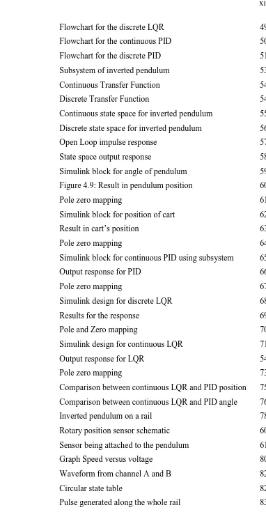
[image:17.612.186.471.484.614.2]PID stands for Proportional-Integral-Derivative. This is a type of feedback controller whose output, a control variable, is generally based on the error between some user defined set point and some measured process variable. Each element of the PID controller refers to a particular action taken on the error. The error is then used to adjust some input to the process in order to its defined set point. The schematic for this problem is depicted as below.
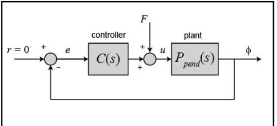
5 The design can be easier to be analyzed by using below figure.
Figure 2.2: Easier schematic
Three parameters must be designed in the PID controller and each parameter has an effect on the error. The transfer function of the PID controller is written as [3]:
= + + .
Where, Kpis the controller gain, Ki is the integral time and Kd is the derivative time. It is important to determine appropriate parameters to guarantee stability and system performance. There are several methods for tuning PID parameters. However, in this study the three parameters of PID controller values are computed by trial and error.
Proportional: Error multiplied by a gain, Kp. This is an adjustable amplifier. In many systems Kp is responsible for process stability. Too low and the PV can drift away. Too high and the PV can oscillate.
Integral: The integral of error multiplied by a gain, Ki. In many systems Ki is responsible for driving error to zero, but to set Ki too high is to invite oscillation or instability.
2.2 LQR Controller
In order to overcome some problems that faced by PID controller, the other type of control methods can be developed such as Linear-Quadratic Regulator (LQR) optimal control. LQR is a control scheme that gives the best possible performance with respect to some given measure of performance. The performance measure is a quadratic function composed of state vector and control input.
Linear Quadratic Regulator (LQR) is the optimal theory of pole placement method. LQR algorithm defines the optimal pole location based on two cost function. To find the optimal gains, one should define the optimal performance index firstly and then solve algebraic Riccati equation. LQR does not have any specific solution to define the cost function to obtain the optimal gains and the cost function should be defined in iterative manner.
LQR is a control scheme that provides the best possible performance with respect to some given measure of performance. The LQR design problem is to design a state feedback controller K such that the objective function J is minimized. In this method a feedback gain matrix is designed which minimizes the objective function in order to achieve some compromise between the use of control effort, the magnitude, and the speed of response that will guarantee a stable system. For a continuous-time linear system described by [4]:
ẋ= +
With a cost functional defined as
= ʃ( ᵀ + ᵀ )
Where Q and R are the weight matrices, Q is required to be positive definite or positive semi-definite symmetry matrix. R is required to be positive definite symmetry matrix. One practical method is to Q and R to be diagonal matrix. The value of the elements in Q and R is related to its contribution to the cost function J. The feedback control law that minimizes the value of the cost is:
= − K is given by
7 And P can be found by solving the continuous time algebraic Riccati equation:
ᵀ + − ᵀ + = 0
The LQR algorithm is, at its core, just an automated way of finding an appropriate state. As such it is not uncommon to find that control engineers prefer alternative methods like full state feedback (also known as pole placement) to find a controller over the use of the LQR algorithm. With these the engineer has a much clearer linkage between adjusted parameters and the resulting changes in controller behavior. Difficulty in finding the right weighting factors limits the application of the LQR based controller synthesis.
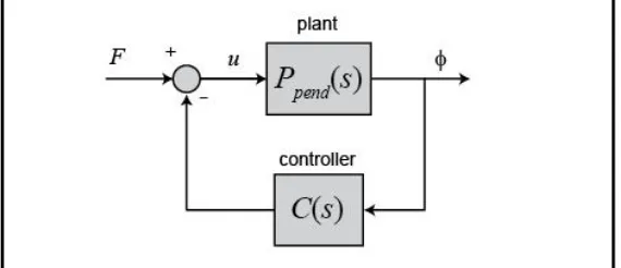
2.3 Inverted Pendulum
It is virtually impossible to balance a pendulum in the inverted position without applying some external force to the system. The problem involves a cart, able to move backwards and forwards, and a pendulum, hinged to the cart at the bottom of its length such that the pendulum can move in the same plane as the cart. That is, the pendulum mounted on the cart is free to fall along the cart's axis of motion. The system is to be controlled so that the pendulum remains balanced and upright, and is resistant to a step disturbance.
If the pendulum starts off-centre, it will begin to fall. The pendulum is coupled to the cart, and the cart will start to move in the opposite direction, just as moving the cart would cause the pendulum to become off centre. As change to one of parts of the system results in change to the other part, this is a more complicated control system than it appears at first glance. The inverted pendulum cart runs along a track. A rotary position sensor measures the cart position from its rotation and another potentiometer measures the angle of the pendulum.
Figure 2.3: Single inverted pendulum
The inverted pendulum is mounted on a moving cart. A servomotor is controlling the translation motion of the cart. That is, the cart is coupled with a DC motor through pulley and belt mechanism. The motor is derived by DC electronics, which also contains controller circuits. A rotary position sensor is used to feedback the angular motion of the pendulum to servo electronics to generate actuating-signal. Controller circuits process the error signal, which then drives the cart through the servomotor. The motion of the cart applies moments on the inverted pendulum and thus it keeps the pendulum upright.
So briefly, the Inverted Pendulum system is made up of a cart and a pendulum. The goal of the controller is to move the cart to its commanded position without causing the pendulum to tip over. In open loop this system is unstable.
The various stages of the work for accomplishing the task of controlling the Inverted Pendulum are as follows:
Modeling the IP and linearizing the model for the operating range.
Analyzing the uncompensated closed loop response with the help of a root locus plot.
Designing the PID controller and simulating it in MATLAB for proper tuning and verification.
9 The problem involves a cart, able to move backwards and forwards, and a pendulum, hinged to the cart at the bottom of its length such that the pendulum can move in the same plane as the cart, shown below. That is, the pendulum mounted on the cart is free to fall along the cart's axis of motion. The system is to be controlled so that the pendulum remains balanced and upright, and is resistant to a step disturbance [5].
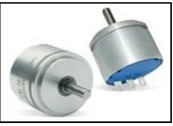
2.3.1 Rotary Position Sensor
[image:22.612.242.414.400.526.2]The model rotary position sensor is a conductive polymer based electronic component which translates angular position into an electrical signal. This sensor can be used in various applications where a user needs to control a variable output such as frequency or volume. It is a 2.1 mm low profile rotary position sensor with a linearity specification of ±2% before and after 1 million rotational cycles. The sensor can function from a temperature range of -40 °C to 120 °C which exceeds the current temperature range available for similar products.
Figure 2.4: Resistive sensor
electronics, appliances, small engines, robotics, motion controllers, automation equipment, electronic instrumentation and medical equipment control panels.
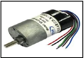
2.3.2 Motor with encoder (SPG30-20K)
[image:23.612.249.408.323.433.2]This DC geared motor with encoder is formed by a quadrature hall effect encoder board which is designed to fit on the rear shaft of Cytron's SPG-30 geared motor series. Two hall effect sensors are placed 90 degree apart to sense and produce two output A and B which is 90 degree out of phase and allowing the direction of rotation to be determined. Please note that the encoder is mounted at the rear shaft, the minimum resolution depends on the motor's gear ratio.
Figure 2.5: DC Geared Motor with Encoder
The disc is painted half white and half black to vary the reflectivity of the surface as it rotates. A reflective pair of light sensors detects this change in light as the motor rotates the disc. An attached microcontroller reads the sensors and can determine the direction and speed of the motor.
11
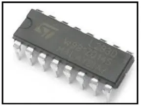
2.3.2 Motor Driver L293
The L293 comes in a standard 16-pin, dual-in line integrated circuit package. There is an L293 and an L293D part number. The D version should be picked because it has built in flyback diodes to minimize inductive voltage spikes. The L293 is an integrated circuit motor driver that can be used for simultaneous, bi-directional control of two small motors.
[image:24.612.255.399.375.484.2]Figure 2.6 shows Motor driver L293D this circuit can be control and drive servo motor by apply the input voltage of 4.8V or 6.0 V. It can be used to control two motor in one time by using principle of H-bridge circuit. The circuit consist two PWM which is right PWM and left PWM to control the speed of servo motor. Each PWM have two motor to produce direction of wheel of robot either forward or backward. When motor 1 is on (bit 1) and motor 2 off (bit 0) the direction of wheel is forward while when the motor 1 is off (bit 0) and motor 2 on (bit 1) the direction of wheel is backward.
Figure 2.6: Motor Driver L293D
Darlington driver or n-channel MOSFET, which is why they cannot be used to reverse a motor.
2.4 MATLAB
MATLAB (matrix laboratory) is a numerical computing environment and fourth-generation programming language. MATLAB is a weakly typed programming language. It is a weakly typed language because types are implicitly converted. It is a dynamically typed language because variables can be assigned without declaring their type, except if they are to be treated as symbolic objects, and that their type can change. Values can come from constants, from computation involving values of other variables, or from the output of a function.
2.4.1 MATLAB Simulink
Simulink is a block diagram environment for multi domain simulation and Model-Based Design. It supports system-level design, simulation, automatic code generation, and continuous test and verification of embedded systems. Simulink is an input/output device GUI block diagram simulator which contains a Library Editor of tools from which we can build input/output devices and continuous and discrete time model simulations. It contains continuous and discontinuous system model elements.
13
2.4.2 M-File
M-files are macros of MATLAB commands that are stored as ordinary text files with the extension ‘m’, that isfilename.m. An M-file can be either a function with input and output variables or a list of commands.
There are four ways of doing code in MATLAB. One can directly enter code in a terminal window. This amounts to using MATLAB as a kind of calculator, and it is good for simple, low-level work. The second method is to create a script M-file. Here, one makes a file with the same code one would enter in a terminal window. When the file is run, the script is carried out. The third method is the function M-file. This method actually creates a function, with inputs and outputs. The fourth method will not be discussed here. It is a way to incorporate C code or FORTRAN code into MATLAB and this method uses .mex files.
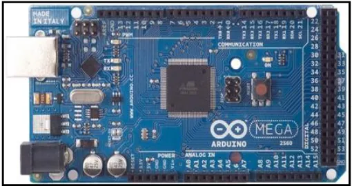
2.5 Arduino MEGA 2560
[image:26.612.203.458.567.702.2]The Arduino Mega 2560 is a microcontroller board based on the ATmega2560. It has 54 digital input/output pins (of which 14 can be used as PWM outputs), 16 analog inputs, 4 UARTs (hardware serial ports), a 16 MHz crystal oscillator, a USB connection, a power jack, an ICSP header, and a reset button. It contains everything needed to support the microcontroller which simply connect it to a computer with a USB cable or power it with an AC-to-DC adapter or battery to get started. The Mega is compatible with most shields designed for the Arduino Duemilanove or Diecimila.
The Arduino Mega 2560 has a number of facilities for communicating with a computer, another Arduino, or other microcontrollers. The Arduino Mega 2560 can be programmed with the Arduino software. The Atmega 2560 on the Arduino Mega comes preburned with a bootloader that allows you to upload new code to it without the use of an external hardware programmer.
2.6 Inverted Pendulum Example in Real Life and Previous Case Study
There are many projects that have the same idea of the inverted pendulum nowadays. There may be some robotic project that also uses the concept of the inverted pendulum as well as the controller that is being fed to the system. The idea of it is applicable on the system that is being design. These references help so much in implementing this project.
2.6.1 Inverted Pendulum Example in Real Life
[image:27.612.112.551.526.710.2]There are so many things in the surrounding that has the same idea as the inverted pendulum. All of these things has also contribute in the making this project. The application of it can give clear information about the process of handling the inverted pendulum.
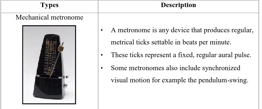
Table 2.1: Inverted Pendulum Example in Real Life
Types Description
Mechanical metronome
A metronome is any device that produces regular, metrical ticks settable in beats per minute.
These ticks represent a fixed, regular aural pulse. Some metronomes also include synchronized
15
Segway PT The Segway PT is a two-wheeled,
self-balancing, battery-powered electric vehicle invented by Dean Kamen. It is produced by Segway Inc. of New Hampshire, USA.
The Segway detects, as it balances, the change in its center of mass, and first establishes and then maintains a corresponding speed, forward or backward. Gyroscopic sensors and fluid-based leveling sensors detect the weight shift.
Loading Crane Crane is a type of machine, generally equipped with a hoist, wire ropes or chains, and sheaves, that can be used both to lift and lower materials and to move them horizontally.
It is mainly used for lifting heavy things and transporting them to other places. It uses one or more simple machines to create mechanical advantage and thus move loads beyond the normal capability of a man.
2.6.2 Previous Case Study
2.6.2.1 LQG/LTR Controller Design for Rotary Inverted Pendulum Quanser Real-Time Experiment
This experiment consists of a rigid link (pendulum) rotating in a vertical plane. The rigid link is attached to a pivot arm, which is mounted on the load shaft of a DC-motor [6]. The pivot arm can be rotated in the horizontal plane by the DC-motor. The DC-motor is instrumented with a potentiometer. In addition, a potentiometer is mounted on the pivot arm to measure the pendulum angle. The principal objective of this experiment is to balance the pendulum in the vertical upright position and to position the pivot arm. Since the plant has two degrees of freedom but only one actuator, the system is under-actuated and exhibits significant nonlinear behavior for large pendulum excursion. The purpose is to design a robust controller in order to realize a real-time control of the pendulum position using a Quanser PC board and power module and the appropriate WinCon real-time software. For the controller design is used a well-known robust method, called LQG/LTR (Linear Quadratic Gauss Ian/Loop Transfer Recovery) which implements an optimal statefeedback. The real-time experiment is realized in the Automatic Control laboratory.
2.6.2.2 DC Motor Controller Using Linear Quadratic Regulator (LQR) Algorithm Implementation on PIC
17 LQR controller by using the MATLAB software. The stable system is got by tuning the Q and R value that can be seen by the simulation.
2.6.2.3 Modeling and Controller Design for an Inverted Pendulum System
The Inverted Pendulum System is an under actuated, unstable and nonlinear system [8]. Therefore, control system design of such a system is a challenging task. To design a control system, this thesis first obtains the nonlinear modeling of this system. Then, a linearized model is obtained from the nonlinear model about vertical (unstable) equilibrium point. Next, for this linearized system, an LQR controller is designed. Finally, a PID controller is designed via pole placement method where the closed loop poles to be placed at desired locations are obtained through the above LQR technique. The PID controller has been implemented on the experimental set up.
2.6.2.4 Real-Time Optimal Control for Rotary Inverted Pendulum
2.6.2.5 Controller Design of Inverted Pendulum Using Pole Placement and LQR
In this paper modeling of an inverted pendulum is done using Euler – Lagrange energy equation for stabilization of the pendulum [10]. The controller gain is evaluated through state feedback and Linear Quadratic optimal regulator controller techniques and also the results for both the controller are compared. The SFB controller is designed by Pole-Placement technique. An advantage of Quadratic Control method over the pole-placement techniques is that the former provides a systematic way of computing the state feedback control gain matrix. LQR controller is designed by the selection on choosing. The proposed system extends classical inverted pendulum by incorporating two moving masses. The motion of two masses that slide along the horizontal plane is controllable.
2.6.2.6 Stabilization of Real Inverted Pendulum Using Pole Separation Factor
Based on the pole placement design technique, a full state feedback controller using separation factor is proposed to stabilize a real single inverted pendulum [11]. The strategy is to start with selection two dominant poles that achieve a certain desired performance, using a separation factor between the selected dominant poles and the other poles to eliminate their effect on the system performance, and finally Ackermann’s formula can be used to calculate the feedback gain matrix to place the system poles at the desired locations. Simulation and experimental results demonstrate the effectiveness of the proposed controller, which offers an excellent stabilizing and also ability to overcome the external resistance acting on the pendulum system.
2.7.7 Modeling and Controller Design of Inverted Pendulum
METHODOLOGY
This research is adopting methods approach involving development and improvement to enhance the overall process of project implementation. The project’s Gantt chart is given in Appendix A. The research is conducting in three phase’s basis. This phase will make sure that the work will be organized based on the scheduled task.
This project is divided into two parts which is hardware and software. Therefore, this chapter will discuss about the process for each parts includes designing, testing, troubleshooting and integrating in order to create one whole system of LQR and PID Controller Design for Inverted Pendulum.
3.1 Familiarization of the System (Phase 1)
In order to implement this project, the first phase that is needed to be concerned is the familiarization of the system. The whole system should be identified and clarified in order to execute the correct process flow of this system.
3.1.1 System Overview
21 to achieve its target. In the meanwhile it will not have too strong oscillation range, too fast speed and angular velocity. When the inverted pendulum system achieves the desired position, it can overcome a range of disturbance and keep balance.
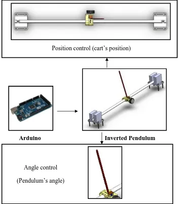
[image:34.612.160.511.164.566.2]Arduino Inverted Pendulum
Figure 3.1: The Block Diagram of the system
Based on the above block diagram, it is shown that there are two elements that need to be controlled in using the inverted pendulum. The first one is the position control by the cart or the system meanwhile for the other one is by controlling the angle of the pendulum. The Arduino Mega in order to interface the software to the hardware so that the inverted pendulum can work as desired.
Angle control (Pendulum’s angle)
3.2 Project Implementation (Phase 2)
The project implementation will covers all of the controllers that will be done in this project. The mathematical model for each of the controller is very important in order to design the controller. The controller itself plays a big role in order to stabilize the inverted pendulum in upright position.
3.2.1 Inverted Pendulum
In this section, two control methods are proposed and explained in details which are PID and Linear Quadratic Regulator (LQR) controllers. Furthermore, the following design specifications have been made to evaluate the performance of both control schemes. The parameters that are used in designing the inverted pendulum are as below:
M mass of the cart 0.208 kg
m mass of the pendulum 0.08 kg
b friction of the cart 0.16 N/m/sec l length to pendulum center of mass 0.382 m
I inertia of the pendulum 12.5e-6 kg*m^2 L
F
Length of the rail
force applied to the cart 0.894m x cart position coordinate
23
Figure 3.2: Single inverted pendulum model
The cart with an inverted pendulum, shown in Figure 3.1, is bumped with an impulse force, F. The dynamic equations of motion for the system, and the pendulum's angle, theta = 0 is linearized. In other words, the pendulum are assume does not move more than a few degrees away from the vertical.
3.2.1.1 Equations of Motion
To derive the suitable mathematical model for an Inverted Pendulum system, Figure 3.2 is considered. Below is the mathematical equation for the system.
Adding all the forces on the cart in the horizontal direction,
ẍ + ẋ + = (1)
Adding all the forces on the pendulum in the horizontal direction,
ẍ + Ӫ − à ² sin = N (2)
Substituting equation (2) in equation (1),
( + )ẍ + ẋ + Ӫ − Ӫ = (3)
Adding all the forces along the vertical direction of the pendulum,
+ cos − = Ӫ + ẍ cos (4)
Considering sum of the moments about the center of gravity (COG) of the pendulum,
− − cos = Ӫ (5)
Now, from equation (4) & (5)
The system under consideration is a non-linear system. For ease of modeling and simulation, it has to take a small case approximation such that the system will be a linear one. The linearization point will be θ = Π
= Π +
ϕis the angle between the pendulum and vertical upward direction. If it is chosen that, ϕ≈0,then cos = -1, sin = -ϕ
So, after linearization equation (6) becomes,
( + ) − = ẍ (7)
And equation (3) becomes,
( + )ẍ + ẋ − =
Here, F is the mechanical force to be applied on the moving cart system. But in real time model it needs to input voltage proportional to the force F. If the input voltage is u, then equation (8) becomes,
( + )ẍ + ẋ − = (8)
3.2.1.2 Transfer Function
The transfer function of a linear, time-invariant, differential equation system is defined as the ratio of the Laplace transform of the output (response function) to the Laplace transform of the input (driving function) under the assumption that all initial conditions are zero.
Transfer function = G(s) = [ ]
[ ]
By using the concept of transfer function, it is possible to represent system dynamics by algebraic equation in s. If the highest power of s in the denominator of the transfer function is equal to n, the system is called an nth-order system [11].
Laplace transform of equation (7)
91
REFERENCES
1. Rowell, Derek and Wormley, David N., System Dynamics: An Introduction, Prentice-Hall, Upper Saddle River, New Jersey, 1997.
2. Magana Me; Holzapfel F, Fuzzy-Logic Control of an Inverted Pendulum With Vision Feedback, IEEE Transactions On Education
3. Norman S. Nice, Control System Engineering, John Wiley & Son, 2000
4. Sontag, Eduardo (1998). Mathematical Control Theory: Deterministic Finite Dimensional Systems. Second Edition. Springer.
5. Ohsumi A, Izumikawa T. Nonlinear control of swing-up and stabilization of an inverted pendulum. Proceedings of the 34th Conference on Decision and Control, 1995. p. 3873–80.
6. Cosmin Ionete, LQG/LTR Controller Design for Rotary Inverted Pendulum Quanser Real-Time Experiment, University of Craiova, Faculty of Automation, Computers and Electronics Department of Automation.
7. Mohd Isa , Nur Iznie Afrah (2008) DC Motor Controller Using Linear Quadratic Regulator (LQR) Algorithm Implementation on PIC. EngD thesis, Universiti
Malaysia Pahang.
8. Ahmad Nor Kasruddin (2007) Modeling and controller design for an inverted pendulum system. Masters thesis, Universiti Teknologi Malaysia, Faculty of Electrical Engineering.
9. Viroch Sukontanakarn and Manukid Parnichkun, Real-Time Optimal Control for Rotary Inverted Pendulum, Mechatronics, School of Engineering and
10. Katsuhiko Ogata, University of Minnesota, A text book of Modern Control Engineering.Prentise Hall, 1994.
11. Amr A. Roshdy,Stabilization of Real Inverted Pendulum Using Pole Separation Factor, College of Mechanical and Electric Engineering Changchun University of Science and Technology.
12. Pankaj Kumar, Modeling and Controller Design of Inverted Pendulum, International Journal of Advanced Research in Computer Engineering & Technology (IJARCET) Volume 2, Issue 1, January 2013
13. H W Broer, I Hoveijn, M van Noort, G. Vegter. The Inverted Pendulum: A Singularity Theory Approach.Journal of Differential Equations, Volume Issue 1, 1 September 1999, Pages 120-149
14. Franklin, Gene F., Powell, David J., and Emami-Maeini, Abbas, Feedback Control of Dynamic Systems, Addison-Wesley, New York, 1994.
15. Katsuhiko Ogata, Discrete Time Control Systems Second Edition, Prentise Hall, 1994.
16. Carlos Aguilar Ibanez, O. Gutierrez Frias, and M. Suarez Castanon, Lyapunov-Based Controller for the Inverted Pendulum Cart System, Springer Journal: Nonlinear Dynamics, Vol. 40, No. 4, June 2005, pp. 367-374.
17. Sergey Edward Lyshevski, Control Systems Theory with Engineering Application, Birkhauser Bostan, 2000.
18. H. J. T Smith, “Experimental study on inverted pendulum in April 1992”. IEEE 1991.
19. Q. G. Chen, N. Wang, S. F. Huang, The distribution population based Genetic Algorithm for parameter optimization PID controller, ACTA Automatic SINICA, vol.31, pp.646-650, 2005
93 21. I.Mizumoto, D. Ikeda, T. Hirahata and Z. Iwai, Design of Discrete Time Adaptive PID Control Systems with Parallel Feedforward Compensator, Proc of 2008
International Symposium on Advanced Control of Industrial Processes, Jasper, Alberta, Canada, May 4-7, pp.212-217, 2008.
22. Ajit K. Mandal, Introduction to Control Engineering, New Age International Publication, New Delhi, 2000, Chapter 13.
23. M. N. Bandyopadhyay, Control Engineering: Theory and Practice, Prentice Hall of India Pvt. Ltd., New Delhi, 2004, Chapter 13
24. James Fisher, and Raktim Bhattacharya, Linear quadratic regulation of systems with stochastic parameter uncertainties, Elsevier Journal of Automatica, vol. 45, 2009, pp. 2831-2841.