Stability Analysis of a Five phase Induction Motor Drive Using Variable Frequency Technique

(1)

Stability Analysis of a Five-phase Induction Motor Drive

Using Variable Frequency Technique

M. S. Alam

1

_{, M. Rizwan Khan}

2,*

1_{Electrical Engineering Section, Aligarh Muslim University, India} 2_{Department of Electrical Engineering, Aligarh Muslim University, India}

Abstract

This paper presents stability analysis of a five phase induction motor drive using different control techniques such as Root locus, Bode plot and Nyquist plot. A dynamic model based on voltage- current and voltage-flux linkage relationship is developed. To evaluate the control performance of the five phase induction motor drive, a linearized model is used. The voltage –flux linkage model is derived from the dynamic model in d-q axes. To evaluate the control performance of the motor small perturbations are applied with the model. Five- phase induction motor drive may become unstable at low values of frequency. Transfer function of the drive is determined at different rotor frequencies and the effect on the stability of the drive is assessed using different control techniques. The value of the rotor frequency at which the drive becomes unstable is reported. The effect of variation of rotor frequency on the performance of the motor drive is analyzed. The analysis is carried out using Matlab codes.

Keywords

Five-phase Induction Motor Drive, Stability Analysis, d-q Axes, Transfer Function, Matlab Codes

1. Introduction

Three-phase induction motor was invented by Russian engineer M.O. Dolivo-Dobrovolsky in 1889. The improvement in the construction materials and design performance of the motor was made for many years. Although there was no change in the fundamental engineering solutions proposed by Dobrovolsky, Machowski et al. [1] has reported that electrical motors consume about 65-70% of energy out of which 90% are induction motors [2]. Induction motors are the essential part of any power system. The dynamics of the induction motor is studied by developing the mathematical model. Stability of the motor means the ability of the drive to retain steady state condition after a small disturbance has occurred. Stability of an induction motor drive is important characteristic which

provides reliability of work. For the normal operation of the motor, steady-state stability is the necessary condition. By placement of Eigen values, the stability analysis of the machine is performed under small perturbations of the machine. Three phase induction motor drive utilizes the voltage- flux linkage model which is derived from the dynamic model in d-q axes [6]. Three phase induction motor utilizes transfer function approach for stability analysis.

High phase induction motor drives are considered for a number of applications such as electric ship propulsion, more electric aircraft and traction applications. High phase induction motor drives are preferred over three phase drive because of reduction in per phase capacity of the drive, reduction in high frequency loss, reduction in the torque pulsation, reduction in the vibration and noise. Stability analysis of the machine was done on the basis of small displacement method for obtaining the linear equations and any one of the conventional technique of the control system may be used. Root locus technique is used to perform the stability study [3]. Stability analysis of a rectifier-inverter induction motor drive is performed by applying the Nyquest stability criterion, two dimensional unstable regions was provided in this paper [4]. Stability study based on Transfer function for the development of controlled current Induction Motor Drives is done by Cornell and Lipo [5]. Evaluation of the control performance of three phase induction motor drive based on conventional techniques is developed by Islam et al.[6]. Regulation of inverter frequency helps in suppression of oscillations of induction motor drive PWM inverters [7]. Based on Liyapunov’s Stability theory, the stability of voltage source inverter and traction induction machine drive feeding in the lead acid traction battery package is analyzed [8]. A mathematical d-q model of six- phase, two pole induction motor in reference frame has been presented [9]. Voltage- flux-linkage model of five-phase induction motor drive is linearized on a small signal perturbation basis at a steady state operating point and a transfer function is derived between input and output. The transfer function is derived between rotor frequency and torque load [10].

(2)

available in detail [11, 12]. The machine model is linearized on a small signal perturbation basis at a steady sate operating point and the transfer function between rotor frequency and stator frequency is derived by varying the rotor frequency and the stability analysis is performed. The stability analysis of five phase induction motor drive is performed using classical methods such as Bode Plot, Nyquist plot and Root locus of control system.

2. Voltage-Flux-Linkage Model

In the modeling of Five-phase induction motor drive, the synchronous reference frame is used as a starting point. In this model some assumptions such as linear inductances, constant resistances, sinusoidal distribution of windings along the circumference of the machine, are adopted. The iron losses, slot harmonics and skin effects are neglected. These alterations do not affect the main characteristics of the motor drive. The flux linkage representation is used in motor drive to highlight the process of the decoupling of flux and torque channels in the induction machine. The stator and rotor flux linkages in the arbitrary reference frame are defined as:

ψ

𝑞𝑞𝑞𝑞 = Ls.Iqs+LmIqr

ψ

𝑑𝑑𝑞𝑞= Ls.Ids+LmIdr

ψ

𝑞𝑞 𝑟𝑟= LrIqr+LmIqs

ψ

𝑑𝑑𝑟𝑟 = LrIdr+LmIds

ψ

𝑥𝑥𝑞𝑞= LlsIxs

ψ

𝑦𝑦𝑞𝑞= LlsIys (1)

ψ

𝑥𝑥𝑟𝑟= LlrIxr

ψ

𝑦𝑦𝑟𝑟=LlrIyr

ψ

𝑜𝑜𝑞𝑞= LlsIos

ψ

or = LlrIor

The q axis stator voltage in the arbitrary reference frame is Vqs= Rs.Iqs+𝜔𝜔𝑟𝑟(Ls.Ids+LmIdr)+ Lm

p

Iqr+Ls

p

Iqs (2)

Where

p

= _{𝑑𝑑𝑑𝑑}𝑑𝑑

Substituting from the defined flux-linkages into the voltage equations yields

Vqs= Rs.Iqs+𝜔𝜔𝑟𝑟

ψ

_{𝑑𝑑𝑞𝑞}+

p

ψ

_{𝑞𝑞𝑞𝑞} (3)

The electromagnetic torque in flux linkages and currents is derived as

.

2 1 1

2 2 2

(

)

(

)

e e e e

m

eo qso dro dso qro

e e e e

m

eo xso yro yso xro

ls lr

L

T

P

D

L

T

P

L L

ψ ψ

=

−

=

−

(4)

(

)

1

₂

r

r e L

d

P

J

f

T T

dt

ω

₊

_ω

₌

₋

(5) Where D = Ls*Lr-Lm2

𝑓𝑓1=friction coefficient

𝑇𝑇𝑒𝑒=electromagnetic torque

𝑇𝑇𝐿𝐿=shaft torque

The induction machine model in terms of the flux linkages described in above section is made use of in this section. The relation between voltage and flux Linkages can be found by expressing the currents in terms of flux linkages. To derive the relation first we have to specify the voltages, currents and flux linkages vectors in an arbitrary reference frame. Suppose the speed of reference frame is 𝜔𝜔𝑐𝑐=𝜔𝜔𝑞𝑞, stator

supply angular frequency in rad/sec and 𝜃𝜃𝑐𝑐= 𝜃𝜃𝑞𝑞

instantaneous angular position in radians.

The relation between the voltage and current is given by

1 2 1 1 1 1 1 1 1 1 1 2 1 1 1 1

1 1 1 1 1 1 1 1 1 1 1 1 1 1

* * 0 0 0 0

* * 0

e

s s s so s m so m

qs e

so s s s s p so m m

ds e

m slo m r m slo r

qr e

slo m m slo r r m

dr e xs e ys e xr e yr

R R L p L L p L V

L R R L L L p V

L p L R L p L V

L L p L R L p V

V V V V

ω ω

  + +

  ₋ _{+ +} ₋

 

  +

 

− − +

  =              

1 2 2 2 2 2 2 2 2 2 1 2 2 2 2 2

2 2 2 2 2 2 2 2 2 2 2 2 2 2

0 0 0

0 0 0 0 * *

e qs e ds e qr e dr e

s s s so s m so m xs

e

so s s s s so m m ys

m slo m r r slo r xr

slo m m slo r r r

I I I I R R L p L L p L I L R R L p L L p I L p L R L p L I

L L p L R L p

ω ω

 

 

 + + 

 

− + + −

 

 ₊ 

 

− − +

 

 

e

e yr

I

                         

(6)

(3)

0

e _e

qs _qs

s m

e _e

ds _s _m _ds

e _e

qr _qr

m r

e _e

dr _m _r _dr

e _e

xs ls _xs

e e ls ys ys e e _lr xr xr e

e _lr _yr

yr

I

L

I

L

I

L

I

L

_I

L

I

L

_I

L

I

ψ





_

_

_





_

_





_

_





_

_





_

_





_

_



_{ = }

_





_

_





_

_





_

_





_

_







































































(7)

This on simplification provides

1

0 0 0 0 0

0 0 0 0

s r s m

so

s r s m

so e

qs r m r s

slo e

ds e

r m r s

qr _slo

e dr

e s s so s m so m

xs

e ls ls lr lr

ys

e so s s

xr

e ls

yr

R L _p R L

D D

R L _p R L

D D

V R L R L _p

V D D

R L R L

V _p

D D

V

R L p L L p L

V

L L L L

V

L R L

V L V ω ω ω ω ω ω ω − + − − +   − ₊     −   ₋ ₊    _{ =} +       − +         2

0 0 0 0

e qs e ds e qr e dr e xs e ys e

s so m m

xr e

ls lr lr

yr

m slo m r r slo r

ls ls lr lr

slo m m slo r r r

ls ls lr lr

p L L p

L L L

L p L R L p L

L L L L

L L p L R L p

L L L L

ψ ψ ψ ψ ψ ψ ω _ψ ψ ω ω ω ω            _{ } _  _{ } _  _{ } _  _{ } _  _{ } _  _{ } _  _{ } _  _{ } _  _{ } _  −   _{ }  _{  }  ₊       ₋ ₋ ₊           (8)

3. Model Linearization

These dynamic equations so obtained are nonlinear. These nonlinear equations cannot be used directly. To make these equations linear perturbation technique is adopted. For solution the equations are to be arranged in state space form. The ideal model for perturbation to get the linearized model is the one with steady-state operating state variables as dc values. This is possible only with the synchronously rotating reference frame model of the induction motor.

r ro r s so s e eo

e

T

δω

ω

δω

ω

δ

δψ

ψ

δψ

ψ

δψ

ψ

δψ

ψ

δ

+

=

+

=

+

=

+

=

+

=

+

=

+

=

+

=

+

=

e dr e dro e dr e qr e qro e qr e ds e dso e ds e qs e qso e qs e ds e dso e ds e qs e qso e qs

v

(9)

The voltages, flux, torque and speed in their steady state are designated by an additional subscript with an ‘o’ in the variables, and the perturbed increments are designated by a δ preceding a variables.

The voltage and flux-linkage vector as follows;

e e e e e e e e qs ds qr dr xs ys xr yr

v v v v v v v v

V

δ δ δ δ δ δ δ δ δ

δψ δψ δψ δψ δψ δψ δψ δψ δψ

 

=  

 

=  

(10) By using perturbation technique and putting all the perturbation equations in the state variables;

(

)

(

)

(

)

(

)

(

)

.

. /

.

. /

e e e e

qso qs s r qso qs

e e e e

so dso ds m s qro qr

V

R L D p

L R D

δ

ψ

δψ

ω ψ

δψ

ψ

δψ

+

=

+

−

+

(4)

(

)

( )

(

)

( )

(

)

( )

/ . . / . . / / . / . / . . / .

e e e e e

qs s r qs so ds s m qr dso s

e e e e e

ds so qs s r ds s m dr qso s

e e e e e e

qr r m qs r s qr slo dr dro r dro s

e e e

dr r m ds slo qr r

V R L D p R L D

V R L D R L D p

V R L D R L

δ

δψ

ω δψ

δψ

ψ

δω

δ

ω δψ

δψ

ψ

δω

δ

δψ

ω δψ

ψ

δω

ψ

δω

δ

δψ

ω δψ

= + + − + = − + + − − = − + + + − + = − − +

(

)

( )

(

)

_{( )}

(

)

_{( )}

/ . . .

e e e

s dr qro r qro s

s s

e e s e m e m e s e m e

xs xs so ys xr so yr yso yro s

ls ls lr lr ls lr

s s

e s e e m e m e s e m

ys so xs ys so xr yr xso

ls ls lr lr ls lr

D p

R L p L L L L L

V p

L L L L L L

R L p

L L L L L

V p

L L L L L L

δψ

ψ

δω

ψ

δω

δ

δψ

ω δψ

δψ

ω δψ

ψ

δω

δ

ω δψ

δψ

ω δψ

δψ

ψ

+ + − +   = + + + +_ + _   + = − + − + − +

( )

(

)

_{( )}

(

)

_{( )}

. . ( ) . e xro s r r

e s e m e e r e m e r e

xr xs slo ys xr slo yr yso yro s r

ls ls lr lr ls lr

r r

e m e m e r e e m e r e

yr slo xs ys slo xr yr yso yro

ls ls lr lr ls lr

R L p

L L L L L

V

L L L L L L

R L p

L L L L L

V p

L L L L L L

ψ

δω

δ

δψ

ω δψ

δψ

ω δψ

ψ

δω δω

δ

ω δψ

δψ

ω δψ

δψ

ψ

      +   = + + + +_ + _ −   +

= − + − + + + (

δω δω

r s)

  −     (12)

(

)

(

)

(

)

1 1 2 , . 2 . . . . . . . . r

r e l

e e e e e e e e

m

e qso dr dro qs dso qr qro ds

e e e e e e e e

m

e xso yr yro xs yso xr xro ys

ls lr

d P

Now J f T T

dt L T P D L T P L L

δω _δω _δ _δ

δ ψ δψ ψ δψ ψ δψ ψ δψ

+ = −

= + − −

In the compact form, equation (12) can be written as

Where;

[

]

[

e

]

yr e xr e ys e xs e dr e qr e ds e qs 2 e yr e xr e ys e xs 1 e dr e qr e ds e qs v v v v v v v v i i i i i i i iI

δ

δω

δ

δω

δ

δω

δ

l s r r T U X = =

Here [X] and [U] represent the state vectors and input vectors, respectively.

3

1 4

1 1 1 1 1 1

0 0 0 0 0 0 0

0 0 0 0 0 0

0 0 0 0 0

0 0 0 0 0 0

0 0 0 0 0

s r s m

so

s r s m

so

r m r s

slo

r m r s

slo

dro qro dso qso

s s so s m so m

ls ls lr lr

so s s s

ls ls

R L _p R L

D D

R L _p R L

D D

R L _{R L p} _C

D D

R L _{R L p C}

D D

K K K K J p B

K R L p L L p L

L L L L

L R L p

L L

ω

ψ ψ ψ ψ

ω ω ω − + − − + − ₊ ₋ − ₋ ₊ − − + = + − + − 7 8

2 2 2 2 2 2

0

0 0 0 0 0

so m m

lr lr

m slo m r r slo r

ls ls lr lr

slo m m slo r r r

ls ls lr lr

yro xro yso xso

L L p

L L

L p L R L p L _C

L L L L

L L p L R L p _C

L L L L

K K K K J p B

ω

ω ω

ψ ψ ψ ψ

(5)

)

1 (

p

P

Q

K

=

−

_;

1

2

1 0 0 0 0 0 0 0 0 0

0 1 0 0 0 0 0 0 0 0

0 0 1 0 0 0 0 0 0 0

0 0 0 1 0 0 0 0 0 0

0 0 0 0 0 0 0 0 0

0 0 0 0 0 0 0 0

1

0 0 0 0 0 0 0 0

0 0 0 0 0 0 0 0 0

s m

ls lr

s m

ls lr

m r

ls lr

m r

lr lr

J

L L

P

L L

J

 

 

=  

 

 

(14)

and

3

1 4

1 1 1 1 1

0 0 0 0 0 0 0

0 0 0 0 0 0

0 0 0 0 0

0 0 0 0 0 0 0

0 0 0 0 0 0

s r s m

so

s r s m

so

r m r s

slo

r m r s

slo

dro qro dso qso

s so s so m

ls ls lr

so s s so m

ls ls lr

sl

R L R L

D D

R L _p R L

D D

R L R L _C

D D

R L R L _C

D D

K K K K B

Q R L L

L L L

L R L

L L L

ω

ψ ψ ψ ψ

ω ω

ω

− −

− ₊

− ₋ −

−

− − −

=

− − −

−

− ₇

8

2 2 2 2 2

0 0 0 0 0 0

0 0 0 0 0

o m r slo r

ls lr lr

slo m slo r r

ls lr lr

yro xro yso xso

L R L _C

L L L

L L R _C

L L L

K K K K B

ω

ω ω

ψ ψ ψ ψ

 

 

 ₋ 

 

−

 ₋ ₋ 

 

 − − − 

 

(15)

Where

2 2

1

( )

m

;

2

( )

m

;

ls lr

L

K

P

K

P

D

L L

=

The system matrix is,

U

R

X

Q

X

P

p

1 *

=

*

+

1 *

(16) Where;

1 2

3 4

1

5 6

7 8

2

1 0 0 0 0 0 0 0 0 0 0

0 1 0 0 0 0 0 0 0 0 0

0 0 1 0 0 0 0 0 0 0 0

0 0 0 1 0 0 0 0 0 0 0

0 0 0 0 0 0 0 0 0 0 0

0 0 0 0 0 0 1 0 0 0 0

0 0 0 0 0 0 0 1 0 0 0

0 0 0 0 0 0 0 0 1 0 0

0 0 0 0 0 0 0 0 0 1 0

0 0 0 0 0 0 0 0 0 0 0

C C

P R

C C

P

−

 

 

 − 

 

 − 

=  

−

 

−

 

 − 

 

(6)

1 dsoe

,

2 qsoe

,

3 droe

,

4 qroe

C

=

ψ

C

=

ψ

C

=

ψ

C

=

ψ

(

)

(

)

(

)

(

)

(

)

(

)

(

)

(

)

5 6 7 8 e e s m yso yro ls lr e e s m xso xro ls lr e e m r yso yro ls lr e e m r yso yro ls lr

L

C

L

C

L

C

L

C

L

ψ





=

_

+

_









=

_

+

_









=

_

+

_









=

_

+

_





(18) The system matrix can be written as;

p[X] [A][X] [B][U]



=



+



(19) Where, 1 * 1 * 1 1 1 R P B Q P A − −       =       = (20)

The second, fifth & sixth column of

[ ]

R₁ matrix is due to

theδVdso,δωs and δTl term respectively. The other input

voltages are zero. The outputs of the machine are taken as incremental currents, incremental torque and incremental speed. The response of machine due to change in each parameter (voltage, load torque and synchronous speed) are elaborated. One quantity is changed at one time. The incremental output, currents torque and speed vectors are;

[

]

[

]

[

]

[

]

[

]

1 0 0 0 0 0 0 0 0

0 1 0 0 0 0 0 0 0

0 0 1 0 0 0 0 0 0

0 0 0 1 0 0 0 0 0

0 0 0 0 0 1 0 0 0

e qso e dso e qro e dro e xso e yso

C X

X

C X

X

C X

X

C X

X

C X

X

C X

δψ



    

=

_{   }

=

 

_{ }







    

=

_{   }

=

 

_{ }







    

=

_{   }

=

 

_{ }







    

=

_{   }

=

 

_{ }







    

=

_{   }

=

 

_{ }







    

_{=  }





[

]

[

]

[

]

[

]

3 3 3 3

0 0 0 0 0 0 1 0 0

0 0 0 0 0 0 0 1 0

0 0 0 0 0 0 0 0 1

0 0 0 0 0

0 0 0 0 1 0 0 0 0

e xro

e yro

e e e e

e dro qro dso qso

r

X

C X

X

C X

X

T

C X

k

X

C X

X

δψ

δ

ψ

δω

 

=



 



    

=

_{   }

=

 

_{ }







    

=

_{   }

=

 

_{ }





   





 

=

_{   }

=

_

−

_

_{ }

   

 

=

_{   }

=

_{ }

(21) Where,

3

L

m

k

P

D

=

This model is derived by the authors which is the major contribution of this paper. The behavior of the motor under steady-state condition can be evaluated by determining the transfer functions of the Induction motor Drive. The generalized transfer function of an induction motor drive is given as.

i i d s s m s m s m s m s m s m s m s m s m m s n s n s n s n s n s n s n s n s n n s u s y ₊ + + + + + + + + + + + + + + + + + + +

= ₉ ₁₀

10 8 9 7 8 6 7 5 6 4 5 3 4 2 3 2 1 9 10 8 9 7 8 6 7 5 6 4 5 3 4 2 3 2 1 ) ( ) ( (22)

4. Simulation Results

With the determination of the transfer function of a five phase Induction motor drive, the control characteristic can also be evaluated. The possible transfer functions for different rotor frequency so obtained are given as:

(7)

76.94 s^3 + 3.979e005 s^2 + 2.157e008 s + 3.896e010

--- s^5 + 702.4 s^4 + 2.783e005 s^3 + 8.199e007 s^2 + 1.37e010 s+ 1.027e012 Transfer function: (for frequency 40 Hz)

8.882e-016 s^4 - 371.9 s^3 - 1.795e005 s^2 - 2.855e007 s- 4.445e009 --- s^5 + 702.4 s^4 + 2.821e005 s^3 + 8.441e007 s^2 + 1.463e010 s + 1.296e012 Transfer function (for frequency 30 Hz)

8.882e-016 s^4 - 218.7 s^3 - 1.232e005 s^2 - 3.679e007 s - 9.934e009 --- s^5 + 702.4 s^4 + 2.939e005 s^3 + 9.206e007 s^2 + 1.753e010 s + 2.122e012 Transfer function(for frequency 23 Hz)

8.882e-016 s^4 - 167.1 s^3 - 9.82e004 s^2 - 3.723e007 s - 1.18e010 --- s^5 + 702.4 s^4 + 3.069e005 s^3 + 1.005e008 s^2 + 2.07e010 s + 3.024e012 The stability analysis of five phase induction motor drive

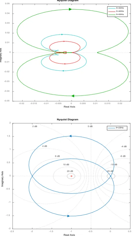
has been carried out for different operating conditions. The transfer functions for different values of rotor frequencies are written above. The four operating conditions adopted for analysis are 50 Hz, 40 Hz, 30 Hz and 23 Hz respectively. Analysis of the transfer functions corresponding to the rotor frequencies is carried out using Nyquest plot, Bode plot and Root locus techniques. Voltage current modal is used for the purpose of analysis. The frequency response for different frequency conditions has been shown in fig. 1, fig. 2, fig. 3 and fig. 4 respectively.

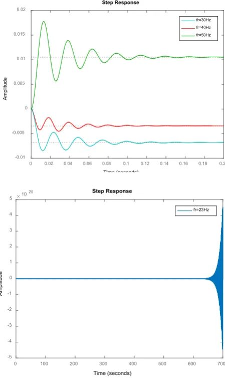
With the decrease in the rotor operating speed the relative stability margin decreases which is clearly seen by these figures. The magnitude of dominant eigen values is also decreases. At a frequency of 23 Hz, the dominant poles crosses the origin, which is the indication of the instability of the drive. The phase margin and gain margin becomes positive at these frequency, so the drive is unstable in fig. 1, at frequency of 23 Hz there are two roots in the positive real part and the encirclement of -1 +j0 plane is not visible, so the drive is unstable in these case. The step response of the drive at different frequency is shown in fig. 2.The response is fast at no load condition. With the corresponding decrease in the rotor speed (decrease in rotor frequency), the response becomes slow, which is the required condition of stability. The induction motor derive becomes unstable at a rotor frequency of 23 Hz. So the five phase induction motor drive is stable at a frequency more than 23 Hz.

Figure 1. Nyquist plot for Five-Phase Induction Motor Drive System

-0.02 -0.015 -0.01 -0.005 0 0.005 0.01 0.015 0.02 -0.05

-0.04 -0.03 -0.02 -0.01 0 0.01 0.02 0.03 0.04 0.05

fr=30Hz fr=40Hz fr=50Hz Nyquist Diagram

Real Axis

Imaginary Axis

-2.5 -2 -1.5 -1 -0.5 0 0.5

-2 -1.5 -1 -0.5 0 0.5 1 1.5 2

-20 dB -10 dB 0 dB

-6 dB -4 dB -2 dB

20 dB 10 dB 6 dB 4 dB

2 dB _fr=23Hz

Nyquist Diagram

Real Axis

[image:7.595.318.550.283.697.2]

(8)

Figure 2. Step response of Five-Phase Induction Motor Drive System

Figure 3. Bode Plots of Five-Phase Induction Motor Drive System

Figure 4. Root Locus contours of Five-Phase Induction Motor Drive System

5. Conclusions

The discussion on the stability analysis of induction motor drive has been carried out in this paper. Linearization of the dynamic model of the drive is done and the state space form of the machine is derived. With the help of this linearized model, we obtained the transfer function which is used to determine the stability of the motor drive under different rotor frequency (rotor speed) conditions. Conventional techniques of control system such as Nyquist plot, Bode plot and Root locus etc. a used for the stability analysis of the five phase induction motor drives. The behavior of the motor load drive is studied using Matlab codes. The rotor frequency is varied from no load (50 Hz) to 23 Hz and behavior of the drive is studied using conventional techniques of control system. At a particular value of rotor speed (rotor frequency=23 Hz) the instability in the behavior of the motor drive is observed. Effect of change of temperature and change in frequency has not been considered in this study. The results based on the voltage- flux linkage model has been reported in this paper.

Appendix

Rating and parameters of the induction motor drive. Five phase, 220 Volts, 50Hz, 4-pole, Stator Resistance, Rs = 6.0 Ohm, Rotor Resistance, Rr = 6.3 ohm, Lm =0.252 H,

Ls=0.252 H, Lr=0.46 H, J=0.03Kg-m2_{β = 0.0 N-m s/rad.}

Nomenclature

A State transition matrix B Control Matrix C Observation Matrix

0 0.02 0.04 0.06 0.08 0.1 0.12 0.14 0.16 0.18 0.2 -0.01

-0.005 0 0.005

0.01 0.015 0.02

fr=30Hz fr=40Hz fr=50Hz

Step Response

Time (seconds)

Amplitude

0 100 200 300 400 500 600 700

-5 -4 -3 -2 -1 0 1 2 3 4 5 10

25

fr=23Hz

Step Response

Time (seconds)

Amplitude

-150 -100 -50 0 50

Magnitude (dB)

101 102 103 104

-360 -180 0 180 360

Phase (deg)

fr=23Hz fr=30Hz fr=40Hz fr=50Hz

Bode Diagram

Frequency (rad/s)

-600 -400 -200 0 200 400 600

-600 -400 -200 0 200 400

600 fr=23Hz

fr=30Hz fr=40Hz fr=50Hz

Root Locus

Real Axis (seconds -1)

Imaginary Axis (seconds

[image:8.595.317.549.80.271.2] [image:8.595.66.291.89.467.2] [image:8.595.59.293.507.700.2]

(9)

D Direct Transmission Matrix di ith column vector of D-matrix

f1 friction coefficient

fs Stator supply frequency (Hz) fr Rotor supply frequency (Hz) H Inertial constant p.u

Ids,Iqs d & q – axis stator current, Amp.

Idr, Iqr d& q – axis rotor current, Amp.

Ixs, Iys stator current in x and y axis, Amp.

Ixr, Iyr rotor current in x and y axis, Amp.

Ios, Ior stator and rotor zero sequence current, Amp.

J total moment of Inertia, Kg-m2

Lm magnetizing inductance per phase, H

Lm1 Magnetizing inductance per phase in q-d axis, H

Lm2 Magnetizing inductance per phase in x-y axis, H

Ls stator inductance per phase, H

Lr rotor inductance, H

Llr stator referred rotor leakage inductance /phase, H

Lls stator leakage inductance per phase, H

P number of poles

p d/dt, differential with respect to time Rs stator resistance per phase, Ohm

Rr stator referred rotor – phase resistance, Ohm

Te electro magnetic torque (N-m)

TL shaft torque (N-m)

Tl Load torque (N-m)

Vds, Vqs d & q -axis voltage of stator, Volts

Vdr, Vqr d & q -axis voltage referred to stator, Volts

ψdr, ψqr d & q –axis rotor flux linkage, V-s

ψds, ψqs d & q –axis stator flux linkage, V-s

ψxs, ψys stator flux linkages in x-y axis, V-s

ψxr, ψyr rotor flux linkages in x-y axis, V-s

ψos zero sequence flux linkage of stator, V-s

ψor zero sequence flux linkage of rotor, V-s

X state variable vector

REFERENCES

[1] J. Machowski, J. W. Bialek and J. R. Bumby, Power system

dynamics: Stability and control, John Wiley and sons, 658, 2011.

[2] Sumper, and A. Baggini, Electrical Energy Efficiency:

Technologies and Applications, John Wiley and Sons, 488, 2012.

[3] R. H. Nelson, T. A. Lipo, P.C. Crause, Stability Analysis of a symmetrical Induction machine”, IEEE Trans. Power Apparatus and System, Vol. 88, No.-11, pp. 1710-1717, Nov. 1969.

[4] T. A. Lipo, P.C. Krause, Stability analysis of a

rectifier-inverter induction motor drive, IEEE Transactions on Power Apparatus and system, vol. 88, No. 1, pp. 55-56,1969.

[5] E. P. Cornell, T. A. Lipo, Modeling and design of Controlled current Induction motor drive system, IEEE Trans. On Industry Applications, Vol. 13, No. 4, pp. 321-330, 1977. [6] S. Islam, F. I. Baksh, S. U. Ahmad and A. Iqbal, Simplified

Stability analysis of a three-phase Induction Motor Drive System, IEEE fifth India International conference on Power Electronics (IICPE-2012) DTU Delhi, India, Dec. 6-8, 2012. [7] N. Mutoh, R. Ueda, K. Sakai et al., Stabilizing control method

for suppressing oscillations of induction motor drive by PWM inverters, IEEE Transactions on Industrial Electronics, vol. 37, No. 1, pp. 48-56, 1990.

[8] Cheng Ximing, Ouyang Minggao, Sun Fengchun, Stability

analysis of the voltage source inverter traction induction machine drive system feeding on a lead-acid traction battery package, Proceedings of the CSEE, vol. 23, no. 10, pp.137-141, 2003.

[9] S. Mandal, Performance analysis of Six-Phase Induction Motor, International Journal of Engineering Research & Tech. (IJERT), ISSN: 2278-0181, Vol. 4 Issue 02, Feb.-2015. [10] M. S. Alam, M. R. Khan, R. Arora, Stability analysis of Five

Phase Induction Motor Drive Using conventional methods, IEEE International conference on Electrical Electronics and Optimization Technique, Chennai, India, March 3-5,2016. [11] B. K. Bose, Modern Power Electronics and AC Drives, PHI

New Delhi, India, 2006.