Sequencing and scheduling oriented customer driven
production planning in CONWIP systems
Taher Taherian
Department of Industrial Engineering Faculty of Engineering
Islamic Azad University,Savehbranch,Saveh,Iran
Samira Bairamzadeh
Department of Industrial EngineeringFaculty of Engineering Tarbiat Moallem University, Karaj,Iran
ABSTRACT
Encountering the backlog is a common phenomenon in make-to-order production systems. The fluctuations in quantity of orders and delivery lead times of customer orders lead to backlog in delivery of orders. What we are going to develop in this paper is identifying the sequencing and scheduling effects on CONWIP parameters. The sequencing and scheduling objective functions exert some specification in system attributes. In this article we will use some sequencing and scheduling objective function to observe the system parameters alterations for example it is important to minimize the number of tardy jobs and total weighted tardiness causes the mentioned backlogs one by one or simultaneously. Because the different importance of orders, we choose a weighting method to calculate the required weights of orders (jobs) in objective functions optimization procedure. Finally we presented a case study using this method in order to increasing the backlogs.
General Terms
Scheduling, Algorithms.Keywords
Backlog reduction, constant work in process, number of tardy jobs, scheduling
1.
INTRODUCTION
For reducing the line stocks in order to achieving the lean production and just-in-time goals, it is vital to move form make-to-stock production systems to make-to-order. Make-to-order production system has fewer inventories in production line but it is very probable to face backlog. What is very important for a customer is less delivery lead time of their orders and get them on time. Kosonen and Buhanist (1995) [1] evaluated the change of a factory into a customer focused lean production system. Chen and Wan (2005) [2] showed the effect of short delivery times in competitive market by comparing two competing MTO firms. Wisner (1995) [3] considering the customer requirements showed the advantages of process oriented manufacturing. Jodlbauer (2007) [4] presented the CONWIP production system parameters include backlog quantity and probability formulas and defined the parameter, work-ahead-window as a period of time that ensure the average quantity of orders during this period is less that available fixed capacity. Zammori et al. (2011) [5] developed a routing flexibility measurement method in manufacturing systems involve CONWIP system. Duri et al.
scheduling problem with dual criteria, the minimization of the total weighted earliness under the influence of minimum number of tardy jobs on a single machine. Soroush (2007) [21] studied a static stochastic scheduling problem on a single machine with random processing times for jobs and arbitrary distributions, and fixed individual weights were imposed on both early and tardy jobs. Molaee et al. (2010) [22] studied the problem of minimization maximum earliness and number of tardy jobs on a single machine simultaneously. Jang and Klein (2002) [23] studied the scheduling problem for the purpose of minimizing the expected number of tardy jobs on a single machine. He et al. (2010) [24] developed a method on the single machine scheduling to minimize the number of tardy jobs with deadlines. Lodree et al. (2004) [25] presented a rule for minimizing the number of tardy jobs in dynamic flow shops. For considering minimizing total weighted tardiness and number of tardy jobs simultaneously, we chose the VNS that is a flexible and easier heuristic to solve the problem. The VNS may give us a non-global optimum but because we want to apply the sequencing and scheduling to evaluate the improvement in backlogs and make some changes in algorithm procedure, so VNS is suitable for us make us less running time in comparison with DP or B&B and more flexibility and complexity in modeling. We try to prove the improvement effects of tardiness objective function optimizations in delivery lead times and backlogs in CONWIP production systems.
2.
MODEL DESCRIPTION
Jodlbauer (2007) considered the CONWIP production system from two viewpoints, customer (market) viewpoint and production (capacity) viewpoint and figured and calculated backlog areas and quantities via a stochastic approach. We are going to unitize a scheduling model to minimize the backlog calculated by Jodlbauer formulas to make more satisfaction of customers.as we know a backlog happens when an order delivered later than its promised date so indeed what brings about the backlog is lateness from due dates. Because the earlier deliverance of orders is not the problem so we consider only the tardiness of order deliverance for improvement. If we minimize the tardiness we can reduce the backlogs so we can model the CONWIP order deliverances as sequencing and scheduling models that the received orders are the jobs must be sequenced and delivery lead times are the due dates. The ready times are the order reception dates. Because the importance of jobs is not equal so we must use the weighted form of tardiness objective functions. What is important for us in minimizing the total weighted tardiness leads to minimizing the backlogs but it is important to maintain the number of tardy jobs fixed or less than primary sequencing.
[image:2.595.316.549.184.316.2]At first a simple example is presented to show the improvement in number of tardy jobs caused by sequence alterations. Table 1 shows some demands for final products during 4 days.
Table 1. Order Quantities During Six Days
Day 1 2 3 4
Orders 200,30,43 28,49,30,29 54 43,19
Assume that all weights for jobs are equal to 1 and the constant production quantity for final product is equal to 120 items per a day. The production chart with primary sequence of jobs (FIFO) will be as following:
Table 2. Tardiness calculations in FIFO sequence.
Job Arrival Day
Completion
Time Due Date Tardiness
1 1 2.66 2 0.66
2 1 2.91 2 0.91
3 1 3.27 3 0.27
4 2 3.5 3 0.5
5 2 3.91 4
6 2 4.16 4 0.16
7 2 4.4 5
8 3 4.85 4 0.85
9 4 5.21 5 0.21
10 4 5.37 5 0.37
In this problem the arrival day or ready times are not important because it is possible to produce the products before their order date and in these cases we deliver the orders since they are arrived. The number of tardy jobs in FIFO sequences of jobs is 8 with total tardiness equal to 3.93 that makes the backlogs about 472 units in total 4 days.
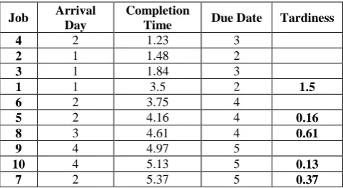
We can exert the first objective function that is minimizing the total weighted tardiness, so the newsequences of jobs ran by computer programmed VNS algorithm has shown in table 3:
Table 3. Total Tardiness optimization using VNS
Job Arrival Day
Completion
Time Due Date Tardiness
4 2 1.23 3
2 1 1.48 2
3 1 1.84 3
1 1 3.5 2 1.5
6 2 3.75 4
5 2 4.16 4 0.16
8 3 4.61 4 0.61
9 4 4.97 5
10 4 5.13 5 0.13
7 2 5.37 5 0.37
Using the total weighted tardiness as first objective function, we will have a new sequencing of orders with 5 numbers of tardy jobs and total tardiness equal to 2.65. In this sort of jobs, we will have total tardiness reduction about %32. There are 3 units reduction in tardy jobs. Although total tardiness reduction is very important objective but maybe it’s better to have a little more quantity of backlog but in less quantity of order.
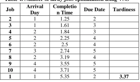
[image:2.595.316.557.457.589.2]Table 4. Number of tardy jobs optimization using VNS
Job Arrival Day
Completio
n Time Due Date Tardiness
2 1 1.25 2
3 1 1.61 3
4 2 1.84 3
5 2 2.25 4
6 2 2.5 4
7 3 2.74 5
8 2 3.19 4
9 4 3.55 5
10 4 3.71 5
1 1 5.35 2 3.37
The minimum number of tardy jobs happens in following sort of jobs via 1 tardy job:
2, 3, 4, 5, 6, 7, 8, 9, 10, 1.
The quantity of backlogs and number of customer orders facing backlog as the results for FIFO, first and second objective function have shown in table 5. The minimum of backlogs and number of tardy orders has shown in bold.
Table 5. Result of three sequencing form of orders FIFO First OF Sec OF Quantity of backlogs 472 318 405
Number of tardy orders 8 5 1
Fig1, shows the Total tardiness and Number of tardy orders within 3 times sequencing alterations.
Fig 1: Total tardiness and number of tardy jobs within 3 types of sequencing.
3.
Combination of Two objective function via
VNS
As it has shown in last parts, minimizing total tardiness led to minimizing the backlogs and some tardy jobs. Also with another objective function we found that we could reduce the number of tardy jobs equal to 1. Although minimizing the backlogs is very important objective but it will not be ideal if we distribute these minimized backlogs to large quantity of customers and make many customers encountered some backlogs which will diminish their satisfaction so finding a method to adjust the total tardiness and number of tardy jobs is very important. To balance the effect of each objective function we can use an efficacy coefficient to push the results
across to one of objective function according to management policies. We choose this coefficient as a decision making weights to sort the orders as alternatives and make the VNS iterations so we define 𝛼 as a coefficient continues between 0 and 1 determines the impact coefficient of total tardiness objective function thus 𝛽 = 1 − 𝛼 is referred to number of tardy job minimization as a coefficient. With a leaner relationship between two mentioned objective function the VNS score will be as following:
Min (total weighted tardiness). 𝛼+ (number of tardy jobs).1 −
𝛼.
So we introduce a VNS algorithm to consider the two objective functions together with a linear relationship between them exerting the impact coefficient.
0- Having n jobs, sort all jobs in FIFO order at first and put the VNS score equal to a very big number like M.
1- substitute (i)th job via (i+1)th job and make new chains of jobs in each substitution for i=1,2, … , n-1 and go to stage. We will have (n-1) chains for each objective function.
2- Calculate the total weighted tardiness (TWT) and number of tardy jobs (NTJ) for each chain of jobs.
3- Normalize 𝑇𝑊𝑇𝑖 and 𝑁𝑇𝐽𝑖 number of tardy jobs resulted for i=1,…,n-1 , using following formula:
𝑇𝑊𝑇𝑖𝑛𝑜𝑟 =
𝑇𝑊𝑇𝑖
Max(𝑇𝑊𝑇𝑖) 𝑖 = 1, … , 𝑛 − 1 (1)
𝑁𝑇𝐽𝑖𝑛𝑜𝑟 =
𝑁𝑇𝐽𝑖
Max(𝑁𝑇𝐽𝑖) 𝑖 = 1, … , 𝑛 − 1 (2)
4- Calculate the VNS score (𝑆𝑖) for each chain as follows:
𝑆𝑖= (𝛼). 𝑇𝑊𝑇𝑖𝑛𝑜𝑟+ 1 − 𝛼 . 𝑁𝑇𝐽𝑖𝑛𝑜𝑟 (3)
5- Sort the VNS scores ascending and choose the minimum chain in scores. If the score is less than previous iteration score go to stage 1 else go to stage 6.
Note: In multiple minimum scores, choose one randomly.
6- The procedure is finished and the selected chain(s) is (are) best solution(s).
The impact coefficient of 𝛼 shows the manager tendency to bold the role of one desired objective function. Whatever this coefficient tends to 1 the manager tendency to bold the total weighted tardiness optimization would increase more than number of tardy jobs minimization and if 𝛼 is selected nearer to 0 it shows the management policy has based on increasing the number of tardy jobs minimization. It is obvious that if 𝛼
0 2 4 6 8FIFO
First Objective
Function Sec
Objective Function
chose equal to 1 the problem turns to just total weighted tardiness optimization problem.
Assuming 𝛼 = 0.35 the new sort of sequencing and scheduling result is as follows:
Table 6. Objective Functions Results via 𝜶 = 𝟎. 𝟑𝟓
Job Arrival Day
Completion
Time Due Date Tardiness
4 2 1.23 3
2 1 1.48 2
3 1 1.84 3
1 1 3.5 2 1.5
6 2 3.75 4
5 2 4.16 4 0.16
10 4 4.32 5
7 2 4.56 5
9 4 4.92 5
8 3 5.37 4 1.37
Considering𝛼 = 0.35, total tardiness was calculated as 3.03 with 3 quantities of tardy orders so total tardiness has increased in contrast with number of tardy order diminution. Fig2 shows the comparison between the four mentioned sequencing of orders in total tardiness and number of tardy jobs.
Fig 2: Objective Function Comparison between 4 sequencingmethods.
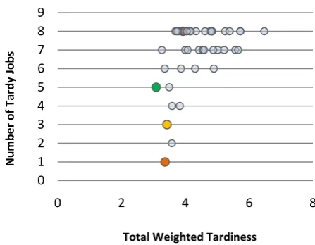
[image:4.595.320.544.86.260.2]As explained, for first iteration in VNS and FIFO sort of jobs, there are some choices to substitute two jobs even if the jobs are not neighbored. Calculation the total weighted tardiness and number of tardy jobs simultaneously, make us capable to compare different states of their combination. To be clearer we can consider different substitutions of jobs and their two mentioned objective functions in one scheme in Fig 3
Fig 3:Possible VNS choices in first iteration of algorithm for simultaneously consideration of two objective
functions.
The abscissa shows total tardiness for each two substitution of jobs and the ordinate show number of tardy jobs for each one.as it has shown, one substitution of jobs has shown via orange point results the minimum number of tardy jobs equal to 1 while its total tardiness is equal to 3.37.it will be obtained by substitution the jobs 1 and 10.If we consider minimum value for total weighted tardiness, it’s referred to the green point and substitution of jobs 1 and 4 via 3.09 but 5 number of tardiness.in FIFO sort of orders and without any substitution, red point, the results will be 8 in number of tardy jobs and 3.93 in total weighted tardiness. Yellow point is a typical point with total weighted tardiness more that minimum value (green point) but 2 unit fewer than green point in number of tardy jobs.
4.
WEIGHT CALCULATION METHOD
To calculate the appropriate weights for each job to use in total weighted tardiness, we make a combination of Entropyweighting method with SAW decision making method. In a routine decision making problems there are some alternatives must be sorted according some criteria using some decision making techniques but if we want to model orders as alternatives and choose some criteria to sort them we can only have a sort of orders not their weights on other words, the difference between our problem and routine decision making problem is we need the weights of alternatives in this problem not criteria. So we used SAW method to calculate the alternatives weights using a decision making matrix. Sofor first step we will make a decision making matrix include i=1,…,m alternatives and j=1,…,n criteria.Shannon’s entropy is a famous method in calculating the weights for an MADM problem especially when acquiring a suitable weight based on the preferences and decision maker experiments are not possible. The original procedure of Shannon’s entropy can be expressed in a series of steps:
1- Normalize the decision making matrix and set 𝑝𝑖𝑗 as following formula:
The raw data are normalized to get rid of anomalies with different measurement scales.
0 1 2 3 4 5 6 7 8 9
FIFO TWT NTJ Combination via α=0.35 Total Tardiness Number of Tardy Jobs
0 1 2 3 4 5 6 7 8 9
0 2 4 6 8
N
u
mb
e
r
o
f Tar
d
y J
o
b
s
Total Weighted Tardiness
𝑝𝑖𝑗=
𝑥𝑖𝑗
𝑥𝑖𝑗 𝑚
2- Compute entropy ℎ𝑗 as following formula:
Where ℎ0 is the entropy constant and is equal to Ln 𝑚 −1 and 𝑝𝑖𝑗. ln 𝑝𝑖𝑗 is defined as 0 if 𝑝𝑖𝑗= 0.
3- Calculate the degree of diversification(𝑑𝑗)
4- Calculate the importance degree of attribute j:
Thus far, we have calculated the weight of each criterion; now we should find a way to reckon the weight of each alternative that’s the order for our problem. Due to this cause, we get help from the method called simple additive weighting (SAW) which is a common decision making technique. In this method we must have the predetermined weights for criteria and the result will be the sequence of the alternatives by arranging the SAW values for alternatives.
5- The values for each alternative can be calculated as:
𝐴𝑖= 𝑤𝑗. 𝑥𝑖𝑗 𝑛
𝑗 =1
(8)
Now the weights of alternatives can be computed as following formula:
𝑤𝑖= 𝐴𝑖𝐴 𝑖 𝑚
𝑖=1 (9)
5.
CASE STUDY
Taherian et al. (2011) presented a case study of TOPCO Automotive Company under FIAT Company license, produced Fiat-Siena and located in southern countryside of Saveh City, Iran and showed that changing the sequences of orders made some decrease in total tardiness that lead to decrease total backlog in CONWIP systems but some factors had been unseenin that problem solving.
1) The weights of each order assumed unique and equal to 1.
2) It only evaluated the total tardiness objective function and had not considered the effect of number of tardiness. The weakness of considering one factor objective function (total tardiness) was that we might reduce total tardiness and increase number of customer orders faces tardiness that is not suitable.
Using the dual objective function presented in this article, we
[image:5.595.312.547.117.326.2] [image:5.595.67.272.200.322.2]resolve the problem and analyze the results again. Also we will calculate the weights of each job and will notice them in solving procedures. The order quantity received from the sale agencies was as follows:
Table 7. Order Received From the Sale Agencies
Day Mon Tue Wed Thi Fri Sat
Date
0
9
/2
2
0
9
/2
3
0
9
/2
4
0
9
/2
5
0
9
/2
6
0
9
/2
7
Tehran 12 7 5
Isfahan 6
Tabriz 5
Mashhad 6 6 7
Saveh 8 3 7
Qom 11 6
Arak 6 5
Bandarabbas
Rasht 5
Shahroud 11 5
Orumia Kermanshah
Tafresh 5
Shiraz 6
Sum 37 25 23 18 23 18
There were 20 jobs available within 6 days period of time. To apply new method, it is necessary for first step to calculate the weights of orders using presented weight calculation methods. Considering 4 criteria include distance between customerand factory (Dist), quantity of demand (Qut), customer degree of impatience (Imp) and permanency of customers (Per), the weights of each criterion has calculated and after that the weights of orders has computed using SAW formulas and has shown in table 8.The total tardiness calculations in FIFO and optimal solution presented in Taherian et al.(2011) so we will present the effect of number of tardy jobs and total tardiness effects simultaneouslyhave presented in this article using the edited form of VNS method and formulas. It’s important to remind the work-ahead-window (WAW)presented by Taherian et al. (2011) prevented capacity problems and gave us a period of time that we could be sure that our capacity was enough to produce demanded orders in average.In This problem theproduction capacity is 6 units per day and the calculated optimal work-ahead-window is 6 days. The calculated weights for 4 criteria using Shannon’s Entropy have shown as follows:
Distance between customer and factory: 0.925 Quantity of demands: 0.016
Customer degree of impatience: 0.005 Permanency of customers: 0.054
Table 8. Weighting Calculation of Orders
Jobs Qut Per Imp Dist Ai Wi
J1,1 12 28 3 120 112.79 0.016
J10,1 11 11 2 800 741.32 0.103
J5,1 8 47 2 7 9.14 0.001
J4,1 6 11 1 1000 926.37 0.128
J5,2 3 47 2 7 9.06 0.001
J13,2 5 16 1 110 102.77 0.014
J3,2 5 14 1 700 648.81 0.090
J14,2 6 12 1 700 648.72 0.090
J7,2 6 22 1 160 149.39 0.021
J2,3 6 24 3 330 306.87 0.042
J6,3 11 25 2 95 89.47 0.012
J1,4 7 28 3 120 112.71 0.016
J4,4 6 11 1 1000 926.37 0.128
ℎ𝑗 = −ℎ0 𝑝𝑖𝑗 𝑚
𝑖=1
. ln 𝑝𝑖𝑗 (5)
𝑝𝑖𝑗=
𝑥𝑖𝑗
𝑥𝑖𝑗 𝑚
𝑖=1 𝑗 = 1, … , 𝑛 , 𝑖 = 1, … , 𝑚 (6)
𝑤𝑗 =
𝑑𝑗
𝑑𝑠 𝑛
J9,4 5 9 1 450 417.12 0.058
J5,5 7 47 2 7 9.13 0.001
J7,5 5 22 1 160 149.38 0.021
J10,5 5 11 2 800 741.22 0.103
J1,6 5 28 3 120 112.68 0.016
J6,6 6 25 2 95 89.39 0.012
J4,6 7 11 1 1000 926.38 0.128
Ej -44.7 -149.8 -11.6 -2597.3 dj 45.063 150.88 12.683 2598.362
Wj 0.016 0.054 0.005 0.926
In FIFO sort of orders and considering job weights for orders total weighted tardiness will be 0.12528 via 7 tardy jobs. The backlog for this value of tardiness will be about 3 cars. You can see the order sequencing of jobs in FIFO sorting in Fig 4.
[image:6.595.306.574.72.175.2]The jobs with tardiness in FIFO sequence has shown in Table 9.
Table 9. Orders facing tardiness in FIFO sort of orders
Sequence Job(order) Name TWT
1 J5, 1 0.00036
2 J4, 1 0.06941
3 J3, 2 0.00747
4 J14, 2 0.02991
5 J7, 2 0.01205
6 J6, 3 0.00360
7 J9, 4 0.00240
[image:6.595.41.295.72.171.2]After applying our method to consider this problem via both total weighted tardiness and number of tardy jobs and assuming 𝛼 = 0.5 to give each objective function a fair importance.
Table 10. Customer order sequencing results considering TWT and NTJ simultaneously using custom VNS via
𝜶 = 𝟎. 𝟓
Jobs Time Due
Time
Compl Time
Tard
ines Weight
Weighted Tardiness
J4,1 0.25 2 1.25 0.016
J5,5 0.2916 6 1.5416 0.103
J5,1 0.3333 2 1.875 0.001
J7,2 0.25 3 2.125 0.128
J5,2 0.125 3 2.25 0.001
J13,2 0.2083 3 2.4583 0.014
J3,2 0.2083 3 2.6666 0.090
J14,2 0.25 3 2.9166 0.090
J1,6 0.2053 7 3.1249 0.021
J2,3 0.25 4 3.3749 0.042
J6,3 0.4583 4 3.8333 0.012
J1,4 0.2916 5 4.1249 0.016
J4,4 0.25 5 4.3749 0.128
J9,4 0.2083 5 4.5833 0.058
J10,1 0.4583 2 5.0416 3.04 0.001 0.00304
J7,5 0.2083 6 5.24999 0.021
J10,5 0.2083 6 5.45833 0.103
J1,1 0.5 2 5.95833 3.96 0.016 0.06336
J6,6 0.25 7 6.20833 0.012
J4,6 0.2916 7 6.49999 0.128
SUM 0.0664
As we can observe the results we can found about %57 tardiness reduction yielded by applying our presented method respect to FIFO sort of jobs. Also the number of tardy jobs has diminished from 7 to 2.
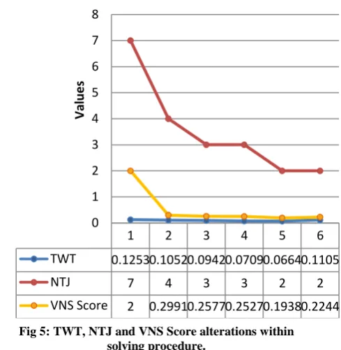
[image:6.595.316.561.244.495.2]The changes in parameters during our custom method using VNS have shown as following:
Fig 5: TWT, NTJ and VNS Score alterations within solving procedure.
VNS continues minimizing TWT and NTJ simultaneously until the VNS score in last iteration is greater than previous score.
6.
CONCLUSION
In this article we evaluated the impact of two sequencing and scheduling objective functions on backlog quantity improvement in CONWIP production system. We considered both of total weighted tardiness and number of tardy jobs during a new heuristic VNS algorithm simultaneously and introduced an impact coefficient to change the weight of each objective function and bold one of them according to management decisions and policies. By creating a program viaBORLAND DELPHI 7 programming language we ran the models and observed the result as VNS score to select the best substitution of jobs according to minimum score. This results aid us to alter the sequences of jobs as the best balance between total weighted tardiness and number of tardy jobs will be resulted. As we showed any reduction in total tardiness leads to reduction in backlog quantities so applying a scheduling and sequencing method could be a good method to increase customer satisfaction by minimizing the probable backlogs or increasing in delivery lead time of orders. In
1 2 3 4 5 6
TWT 0.12530.10520.09420.07090.06640.1105
NTJ 7 4 3 3 2 2
VNS Score 2 0.29910.25770.25270.19380.2244 0
1 2 3 4 5 6 7 8
Val
u
e
s
J10, 1
24 Day 1
Day 2 Day 3 Day 4
J1, 1
J5, 1 J5, 2
J7, 2 J1, 4
Fig. 4. Order Sequencing Scheme in FIFO sort
J4, 1 J13, 2 J3, 2
J14, 2 J2, 3 J6, 3
J3, 2
J6, 3 J4, 4 J9, 4
J5, 5 J7, 5 J10, 5 J1, 6
J6, 6 J4, 6
[image:6.595.48.287.448.551.2]future we can apply the sequencing and scheduling methods on more complex production systems as pull or push or pull-push systems like Kanban and etc.
7.
ACKNOWLEDGEMENT
The authors are grateful to the reviewers for their useful suggestions, which highly contributed to improve the readability and the value of the paper.
8.
REFERENCES
[1] Kosonen, K. and Buhanist, P. 1995. Customer focused lean production development. International Journal of Production Economics 41 (1), 211–216
[2] Chen, H. and Wan, Y-W. 2005. Capacity competition of make-to-order firms. Operations Research Letters 33 (2), 187–194.
[3] Wisner, J.D. andSiferd, S.P. 1995. A survey of US manufacturing practices in make to order machine shops. Production and Inventory Management Journal 36 (1), 1– 7.
[4] Jodlbauer, H. andStocher, W. 2007. Little’s Law in a continuous setting. International Journal of Production Economics 103 (1), 10–16.
[5] Zammori, F., Braglia, M. and Frosolini, M. (2010). CONWIP card setting in a flow-shop system with a batch processing machine. International Journal of Industrial Engineering Computations, 2 (2011) 593–616.
[6] Duri, C., Frein, Y. and Lee, H.S. 2000. Performance evaluation and design of a CONWIP system with inspections. International Journal of Production Economics 64 (1), 219–229.
[7] Braglia, M., Frosolini, R., Gabbrielli, R. and Zammori, F. 2010. CONWIP card setting in a flow-shop system with a batch processing machine. International Journal of Industrial Engineering Computations, 2, 1–18.Cheng, H.; Lio, H. (2010).
[8] Erel, E. and Ghosh, B.2007. Customer order scheduling on a single machine with family setup times: Complexity and algorithms. Applied Mathematics and Computation, 185 (7) 11–18.
[9] Sheng,Y.andLiu,H. 2009. Improving the delivery efficiency of the customer order scheduling problem in a job shop.Computers & Industrial Engineering 57 (9) 856–866.
[10]Kirlik, G. and Oguz, C.2012.A variable neighborhood search for minimizing total weighted tardiness with sequence dependent setup times on a single machine. Computer & Operations Research. 39(7) 1506-1520. [11]Chou, F.D.2009.An experienced learning genetic
algorithm to solve the single machine total weighted tardiness scheduling problem. Expert Systems with Applications. 36(2) 3857-3865.
[12]Wang, X. and Tang, L.2009.A population-based variable neighborhood search for the single machine total weighted tardiness problem. Computers & Operations Resarch. 36(6) 2105-2110.
[13]Wang, G. and Cheng, E. 2007. Customer order scheduling to minimize total weighted completion time. Omega, 35 (7) 623 – 626.
[14]Volgenant,A. and Teerhuis, E. 1999. Improved heuristics for the n-job single-machine weighted tardiness problem. Computers & Operations Research, 26 (1) 35-44. [15]Cheng, T.C.E., Yuan, J.J. and Liu Z.H. 2005. Single
machine scheduling to minimize total weighted tardiness. European Journal of Operational Research, 165:423-443, 2005.
[16]Congram, R.K., Potts, C.N. and Velde D. 2002. An iterated dynasearch algorithm for the single-machine total weighted tardiness scheduling problem. INFORMS Journal on Computing. 14(1):52-67, 2002.
[17]Taherian, T., Mohammadi, M. and Bairamzadeh, S. 2011. A Scheduling Based Backlog Reduction Method in CONWIP Production Systems. International Journal of Computer Applications, (0975 – 8887) 32– No.5. [18]Du, .J. and Leung, Y.T.1990. Minimizing total tardiness
on one machine is NP-hard. Mathematics of Operations Research, 15:483-495, 1990.
[19]Lee, J-Y. and Kim, Y-D. 2012. Minimizing the number of tardy jobs in a single-machine scheduling problem with periodic maintenance. Computers & Operations Research. 39(9) 2196-2205.
[20]Wan, G. and Yen, B.2009. Single machine scheduling to minimize total weighted earliness subject to minimal number of tardy jobs. European Journal of Operational Research. 195(1) 89-97.
[21]Soroush, H.M. 2007. Minimizing the weighted number of early and tardy jobs in a stochastic single machine scheduling problem. European Journal of Operational Research. 181(1) 266-287.
[22]Molaee, E. and Moslehi, G. 2010. Minimizing maximum earliness and number of tardy jobs in the single machine scheduling problem. Computers & Mathematics with Applications. 60(11) 2909-2919.
[23]Jang, W. and Kelin, C.M. 2002. Minimizing the expected number of tardy jobs when processing times are normally distributed. Operations Research Letters. 30(2) 100-106. [24]He, C., Lin, Y. and Yuan, J. 2010. A note on the single
machine scheduling to minimize the number of tardy jobs with deadlines. European Journal of Operational Research. 201(3) 966-970.

![Ethyl 3 [6 (4 methoxybenzenesulfonamido) 2H indazol 2 yl]propanoate monohydrate](data:image/gif;base64,R0lGODlhAQABAIAAAP///wAAACH5BAEAAAAALAAAAAABAAEAAAICRAEAOw==)