Numerical Investigation of Three-dimensional
Turbulent Wind Flow around Two Square
Buildings with Hip Roofs
J. Venetis
School of Applied Mathematics and Physical Sciences, National Technical University of Athens, Greece
Copyright©2019 by authors, all rights reserved. Authors agree that this article remains permanently open access under the terms of the Creative Commons Attribution License 4.0 International License
Abstract
This computational work aims at studying the three – dimensional turbulent wind flow around two square buildings with pyramid roofs of trivial architectural forms for an arbitrary geographical location. The overall investigation substantially reduces to the fundamental problem of an external three – dimensional turbulent flow field past a mounted obstacle of predefined shape. The novelty of this research is that the independency of the numerical solution for any possible distribution of mesh points was demonstrated in a theoretical manner without the necessity of changing the original grid with simultaneous repetition of the computational process.Keywords
Turbulent Flow, Mounted Obstacle, Finite Volume Method, Voronoi Diagram, Delaunay Triangulation1. Introduction
It is well known that the governing differential equations of any fluid flow, laminar or turbulent, can be solved analytically only for a limited number of simple flow cases of little interest to a mechanical, hydraulic or chemical engineer. The difficulty of solving analytically the momentum conservation equations is due to the form of the terms of acceleration of transfer, which unfortunately are non-linear terms. Nonetheless, exact solutions can generally be achieved for problems where the conditions of the acceleration transfer are zero, e.g. Couette flow, Poiseuille flow, flowing into porous media.
In most practical problems encountered by an engineer, such as the design of a ventilation system of a building, the differential equations describing the air transport are not linear, so there is no analytical solution of closed form. One has to resort to numerical methods.
By means of computational methods, the differential
equations characterizing a flow are approximated by algebraic equations describing the characteristic flux sizes, not across the entire flow field but at specific points (meshpoints), all of which synthesize the numerical grid.
Numerical equations consist of a system of equations that form the basis of any computational code and the solution of which determines all sizes that characterize a flow, velocity field volumetric flow,
Computational methods are generally divided into boundary element methods (BEM) and Domain Discretization methods. The latter are in turn divided into Finite Differences, Finite Element (FEM), (with linear, nonLinear and stochastic elements) and Finite Volume methods.
In the meanwhile, during the last four decades, a large amount of valuable research work has proved that air movement in buildings can be predicted in a reliable manner via Domain Discretization methods.
benefit for building-design studies since knowledge on the airflow structure, and hence thermal comfort indices, is provided before the construction of a building. Nonetheless, there are still particular issues that need to be addressed, such as the adopted assumptions, the suitability of the selected turbulence model, the size and type of the computational domain, the spatial discretization and handling of boundary conditions. More importantly, there is the need for an identification of the different “mathematical settings” which must be applied for the simulation of mechanical and natural ventilation. Additionally, since recent published investigations reveal important differences on thermal comfort predictions between mechanical and natural ventilation, any proposed approach of calculating thermal comfort using CFD must be clarified and justified.
The physical aspects of any fluid flow are generally governed by three fundamental principles: (a) Mass conservation, (b) Energy conservation, (c) Newton’s second law for momentum conservation and (d) chemical species conservation. These fundamental principles can be expressed in terms of basic mathematical equations which in their most general form are either integral or partial differential equations. CFD is the art of discretizing these equations to general algebraic formulations, which are then solved to obtain numbers of the flow-field values, at discrete points in space and time, which correspond to the dependent variables of the flow Ref. [1]; Ref. [2]; Ref. [3].
For flows of practical interest, such as airflow in indoor environments, the flow is, in general, turbulent. Air flow within building spaces is a three-dimensional, highly unsteady flow, which contains a great deal of vorticity. The existing vortex stretching is one of the principal mechanisms by which the intensity of turbulence is increased, thus it governs the rate of conserved quantities’ mixing [4]. When the flow is turbulent then either a turbulence model must be used, which leads to additional equations, or special assumptions must be made about the magnitude of the diffusion effects brought out by turbulence. The most trivial group of partial differential equations usually used in literature for building airflow CFD modelling consists of the conservation of mass, momentum, energy, concentration of chemical species and turbulence parameters. All the governing conservation equations can be expressed in the following general form [1]:
𝜕(𝜌𝜑)\𝜕𝑡+𝑑𝑖𝑣(𝜌 ⋅ 𝑢 ⋅ 𝜑 − 𝜞φ⋅ 𝑔𝑟𝑎𝑛𝑑𝜑)=Sφ (1) where ρ is the density of air or mixture (if chemical species are present), t is the time, uis the velocity vector, Γφ is the diffusion coefficient of the transported quantity, Sφ is the source or sink term and φ is the general transported quantity, i.e. 1 for continuity, ux,uy ,uz for momentum in the
three space directions (in case of Cartesian coordinates), temperature T (or enthalpy h) for energy and Ci for
concentration of chemical species i (for example moisture or pollutants), while turbulence transported quantities
depend on the selected turbulence model. The corresponding diffusion coefficients for each dependent variable solved are briefly reported in references Refs. [1-5].
Evidently, the above fundamental equations are nonlinear in nature and cannot be solved analytically. To confront this issue, CFD provides a transformation of these equations to a system of algebraic equations which can be solved by means of numerical analysis techniques. An iterative procedure is followed, whereby the equations are successively re-linearized and solved until the solution to the original numerical form of the equations is attained. A wide variety of discretization methods exist to transform these equations into algebraic linearized ones.
In general, these methods can be divided into three categories [5]:
Finite-Difference Method (FDM). This method is widely used in CFD applications due to its computational and conceptual simplicity. According to the FDM a flow-field variable is discretized in terms of Taylor’s series expansion about a (grid) point defined by the variable’s either-side derivatives.
Finite-Volume Method (FVM). The algebraic difference equations are formulated by applying the conservation laws directly to a small control volume (grid-cell). In opposition with FDM, it has the advantage of the flexibility of the boundary shape of the computational cells, as the conservation laws apply irrespective of shape. Finite-Element Method (FEM). The method is
formulated so that it minimizes the weighted residual (Galerkin residuals) over the flow field. As this method uses unstructured meshes consisting of cells of different topologies (triangles or quadrilateral for two dimensional meshes), very complex geometries can be handled adequately. Now, in more specific approaches to flows past mounted obstacles, a detailed study on turbulent flow past a surface-mounted cube with two-layer turbulence models was carried out by Lakehal and Rodi in Ref. [6]
In addition, a study numerical study on turbulent flow around a wall-mounted cube is presented in Ref. [7].
Moreover, referring to the prediction of air properties’ distribution within ventilated pilot or real-scale buildings, using CFD methods an excellent review work was carried out by Stavrakakis et al. [8].
On the other hand, the establishment of Finite Volume Method has been made on the basis of the following fundamental steps [9].
The calculation field is divided into a number of control volumes each enclosing a node.
The discretization of the transport equation is achieved based on the following assumptions:
Uniform distribution of the different quantities in the control volume.
Uniform distribution of different quantities on the control volume fronts.
First-order approach with ascending differences in the term of time derivative.
In the calculation of flows through the surfaces of the control volume is made in trying to fulfill the conservative property, so its balance of natural quantity to apply around each finite area and not one point only.
In the meanwhile, a Delaunay triangulation is the straight-line dual of a Voronoi diagram [10]. This one to one mapping between a Voronoi diagram and a Delaunay triangulation guarantees that the resultant truss after the triangulation of a surface cannot behave as an infinitesimal mechanism from kinematical viewpoint [11].
On the other hand, in Ref. [12] a rigorous proof that along an arbitrary streamline of a three – dimensional incompressible flow field, Navier – Stokes equations reduce to Euler equations, i.e. the viscous terms are able to be eliminated. In this framework, one may conclude that along the streamline network of such a flow field Navier – Stokes equations are rendered independent of Stokes constitutive relation. In this context, given that Euler equations arise automatically from Newton’s Second Law, one may deduce that for any incompressible flow field of a Newtonian fluid, Navier – Stokes equations can be considered somewhat equivalent to this Axiom.
Besides, in Ref. [13] a rephrased form of the system of mass and momentum conservation equations for a generic type of a three dimensional, unsteady, viscous flow according to Lagrangian formalism for the fluid motion was performed.
Concurrently, in Ref. [14] air flow past isolated gable-roof buildings with different roof pitches was examined in a thorough and effective manner, whilst for a detailed technical review of building-mounted wind power systems one may refer to [15].
In Ref. [16] a valuable CFD simulation of cross-ventilation for a generic isolated building took place. In Ref. [17], a considerable analysis of airflow over building arrays for assessment of urban wind environment was carried out. The current investigation, aims to study the three – dimensional turbulent wind flow around two square buildings with pyramid roofsof trivial architectural forms for an arbitrary geographical location. The novelty of this work is that the independency of the numerical solution for any possible distribution of mesh points was demonstrated in a theoretical manner without the necessity of changing the original mesh with simultaneous repetition of the computational process.
2. Construction of the Flow Model
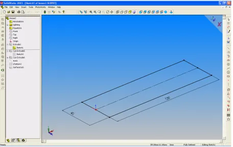
For the construction of the flow model, the Solidworks design software is used. Solidworks is a mechanical CAD program of 3D geometry. In the case we study; the flow model consists of two houses which are placed in a “simulated aerodynamic tunnel”, which from Thermodynamics viewpoint is an open thermodynamic system. A user of Solidworks, has the ability to define the dimensions of the tunnel and the dimensions of the houses. In addition, for houses outside the basic exterior dimensions the program also defines the slope of their roofs.Let us initiate the design by creating the basis of the “simulated aerodynamic tunnel”, (40mX120m) [see Fig. 1] by the following commands
Figure 1. Basis of the “simulated aerodynamic tunnel” The height is created by the following command: "D1@Extrude1" = 40
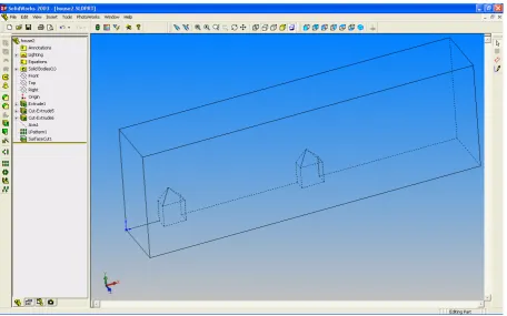
Fig. 2 illustrates the “simulated aerodynamic tunnel”.
[image:4.595.71.528.78.367.2]"D1 @ Sketch3" = 8 "D2 @ Sketch3" = 8
and the distance from the entrance to the tunnel. "D3 @ Sketch3" = 16
Then, with the help of “sketch3” we remove material from our model with equal volume to that of the house. "D1@Cut-Extrude5" = 8
Figure 3. Design of first building
We also build the roof of the house by tilting the vertical with the cut-extrude6 "D3@Cut-Extrude6" = 45
[image:5.595.84.513.154.427.2]For the second house we simply copy the first 50m with the help of Lpattern1 "D3@LPattern1" = 50 "D1@LPattern1" = 2 (Number of copies)
Figure 5. Creation of second house
[image:6.595.69.526.108.391.2] [image:6.595.71.528.440.725.2]In our example, the problem is symmetric, so one may simplify it by subtracting half of surface via command “Cut1” [see Fig. 6]:
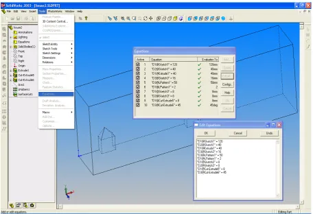
To facilitate the user, the variables can be defined as shown below [see Fig. 7]: (Tools → Equation: Edit all):
"D1 @ Sketch1" = 120: Tunnel length "D2 @ Sketch1" = 40: Tunnel width "D1 @ Extrude1" = 40: Tunnel height
"D3 @ Sketch3" = 16: House distance from tunnel entrance "D3 @ LPattern1" = 50: Distance of 2nd house
"D1 @ LPattern1" = 2: Number of copies "D1 @ Sketch3" = 8: House length "D2 @ Sketch3" = 8: House width "D1 @ Cut-Extrude5" = 8: House height "D3 @ Cut-Extrude6" = 45: Roof Angle
Figure 7. Definition of variables
Now, let us denote that Gambit is a “commercial” grid generator and includes only few (relatively standard) algorithms. New methods are slow to gain robustness and generality and therefore are not directly available.
In the environment of Gambit, one has the ability to construct the solution grid for a given geometry in order to then introduce it into the fluent computational fluent code for the resolution process.
The grid is constructed by selecting the number of nodes for each edge of the geometry or by specifying the width of the distance between them. In addition, in regions where geometry changes (e.g. edges) are strongly altered, local grid densification is performed in order to have more accuracy when solving the problem.
To build a grid on a surface, we first need to determine the number of nodes on each of its sides. So by going to the
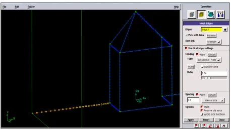
choice of Gambit → Mesh Edges, we may choose the sides we want and then shape the values of the Spacing and Grading
[image:7.595.70.527.108.420.2]Figure 8. Construction of number of nodes on the vertical sides of the house
Then the following figure below shows the local thickening of the grid in the areas before and after the first house during the wind flow. Specifically, in the Grading field, click on Apply and give the value 1.04 to the Ratio parameter, which specifies the rate at which the distance between the nodes increases. [see Fig. 9].
Figure 9. Local Grid Compaction - Enter values in Gambit
[image:8.595.71.528.78.356.2] [image:8.595.69.528.419.678.2]Figure 10. Densification of number of nodes in the middle distance of houses
Similarly, the number of nodes for each of the sides of our geometry is chosen, so the final form of the computational path is shown in below. [see Fig. 11]:
Figure 11. Final Configuration of number of nodes
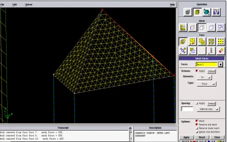
The creation of the grid for the surfaces of the script follows. Select the Mesh area in the Gambit and then click Face. We choose the following [see Fig. 12]:
Elements → Quad (rectangular cells) Type → Map
[image:9.595.69.530.405.631.2]Figure 12. Grid construction on the input surface of the solution loop For the roofs of the two houses we will use triangular cells, so we have [see Fig. 13]: Elements → Tri
Type → Pave
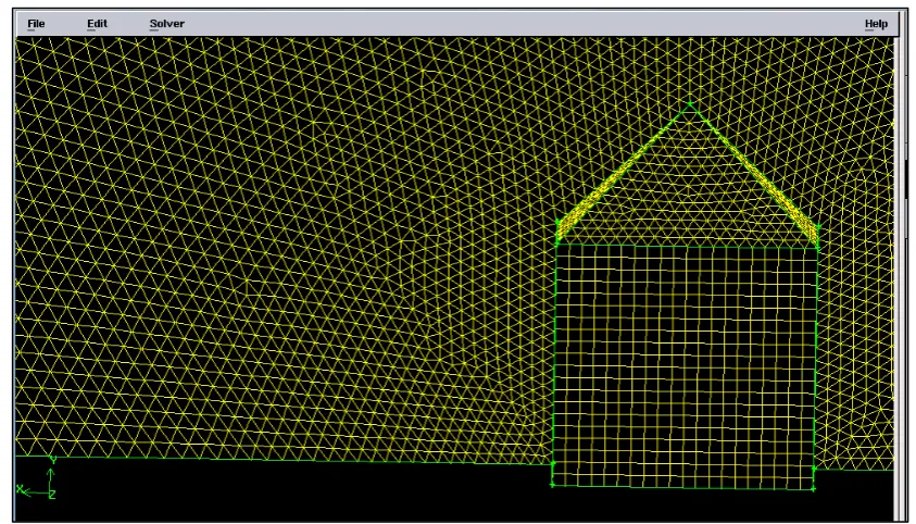
[image:10.595.74.527.448.732.2]Triangular cells will be used for the roofs of the two houses, so we have[see Fig. 14]: Elements → Tri (triangular cells)
[image:11.595.77.518.122.371.2]Type → Pave
Figure 14. Final form of mesh on the surfaces of the solution space
The triangles meet the Delaunay condition [Fig. 15]. The validity of the above statement is supported by the fact that since each roof behaves as a rigid body; apparently any triangulation of its surface corresponds to a kinematic determinate plane truss.
After the mesh construction has been completed on one of the surfaces of the computing space, the final mesh is constructed in this volume by going to the Mesh field and selecting Volume Elements [see Fig. 16]:
Elements → Tet / Hybrid Type → TGrid
[image:11.595.86.508.486.727.2]Figure 16. Final grid
The above final volume is the one that will be introduced to Fluent [20] for the resolution process.
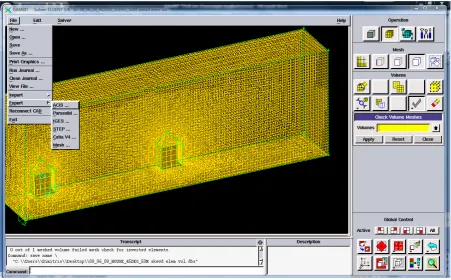
However, Fluent is not able to recognize .DBS files like those that save Gambit [20]. In this context, we need to create an MSH file, which is read by Fluent. [See Fig. 17]:
[image:12.595.72.524.439.719.2]As previously mentioned, the Gambit Design Tool was used to construct the grid in the required geometry of the problem, to follow the solution using the Fluent Computational Fluid Engineering Code. Evidently, Gambit software has saved the file with the geometry and grid of the .msh solution. The introduction of data into Fluent has been made via the following Path:
File → Read → Mesh and the name of the .msh file. Then check the grid to investigate its quality and identify possible errors.
Mesh → Check Mesh Check Domain Extents:
x-coordinate: min (m) = -1.600000e+001, max (m) = 1.040000e+002
y-coordinate: min (m) = 0.000000e+000, max (m) = 4.000000e+001
z-coordinate: min (m) = -2.981556e-016, max (m) = 2.000000e+001
Volume statistics:
minimum volume (m3): 1.855889e-003 maximum volume (m3): 6.894774e-001 total volume (m3): 9.540267e+004 Face area statistics:
minimum face area (m2): 2.388392e-002 maximum face area (m2): 1.635134e+000 Checking number of nodes per cell. Checking number of faces per cell. Checking thread pointers.
Checking number of cells per face. Checking face cells.
Checking cell connectivity. Checking bridge faces. Checking right-handed cells. Checking face handedness. Checking face node order.
Checking element type consistency. Checking boundary types:
Checking face pairs.
Checking periodic boundaries. Checking node count.
Checking nosolve cell count. Checking nosolve face count. Checking face children. Checking cell children. Checking storage. Done.
Additional checks can be made using the following Paths:
Mesh → Info → Quality → Size→ Zones
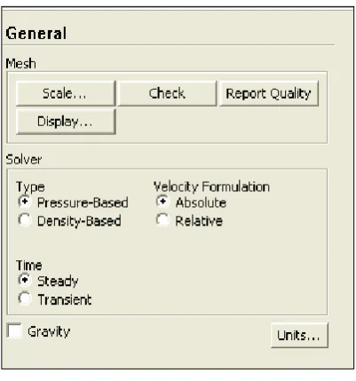
Here are some basic parameters to solve the problem [see Fig. 18]:
[image:13.595.321.522.77.292.2]Define → General
Figure 18. Definition of the parameters
[image:13.595.304.537.395.613.2]We will then turn on the Modes, which are necessary for this problem. Only the flow consistency mechanism is activated, while the other Models are set off. For example, if we wanted to look at the change in temperatures, we would have to activate the Energy mechanism too. [see Fig. 19].
Figure 19. Definition of turbulence model
Figure 20. Definition of wall functions
From the Gambit, the computing space is defined as FLUID, but the properties of the window materials have not been determined. Material or material is selected as “air”. Fluent features a range of Database libraries with a variety of materials depending on the problem of resolution in each case.
So let us follow the path (Path): Define → Materials → Fluid and select air as fluid or medium.
Below is the definition of the boundary conditions of our problem. (Define → Boundary Conditions)
In particular, for the walls, by clicking the wall all → Edit, we determine the roughness of these, if they are moving or not, and their behavior in terms of shear stresses. [see Fig. 21].
In the Thermal, Radiation, Species, DPM, Multiphase, and UDS parameters, there is no need to specify a factor, since the corresponding resolution models are initially disabled. Here is the determination of the boundary conditions for the input of the computing space (velocity inlet). It is assumed that the air enters vertically into the flow field with a uniform profile. It is selected as Velocity Specification Method →Normal to Boundary, and 5m / sec is set as input speed. Note that if we wanted to introduce the air with some inclination, we would choose Velocity Specification Method →Components and we would give values for speed in each of the X, Y, Z axes. The determination of turbulence is done by selecting as Intensity and Hydraulic Diameter, where we give the values 10 and 40 for the turbulence and Hydraulic Diameter respectively. [see Fig. 22]
Likewise, for Thermal, Radiation, Species, DPM, Multiphase, and UDS, there is no need to define a factor, since the corresponding resolution models are initially disabled. The following is the determination of boundary
conditions for outflow. In our problem we do not need to specify any extra data for the output and also the value of the flow rate weighting is set to 1. If we had a second exit, then we would set a value other than the unit, depending on the distribution in each of them. [see Fig. 23].
[image:14.595.306.536.232.478.2]Having defined the boundary conditions of our problem, we will define some of the parameters that are necessary in solving.First we set values for under-relaxation factors [see Fig. 24]. These coefficients express the value that will take a certain size after each iteration in relation to the previous value. The closer to 1 is this factor, the faster the convergence of that size.
[image:14.595.306.535.499.734.2]Figure 21. Definition of boundary conditions
Figure 23. Flow rate weighting
Figure 24. Solution controls
[image:15.595.305.537.80.315.2]For the solution methods, let us preserve the default values [see Fig. 25]
Figure 25. Default values
Figure 26. Run calculation
Finally, in order to begin the solution procedure, let us apply the route:
Solve → Run Calculation,
Here, as the number of iterations let us set the value 500 [see Fig. 26].
Before we proceed to the results of the resolution, we report that we are gradually saving our file by selecting the path:
File → Write → Case and enter a filename (for example as 08_06_08_HOUSE_45DEG_50M)
Now, if we want to run our file, we shall follow the path: File → Read → Case
Next, one may select the file name.
We also have the ability to save the results of the resolution process by a number of iterations. This is done by going to Solve → Calculation activities → Settings, where we define the number of iterations and give a .dat file name.
Returning to solve the problem and clicking Calculate, we notice that after 143 iterations our solution has converged [see Fig. 27]. The following message appears on the screen:
iter continuity x-velocity y-velocity z-velocity to epsilon time / iter
143 solution is converged
[image:15.595.60.289.471.720.2]Figure 27. Evolution of residuals at resolution
[image:16.595.68.527.78.340.2]Here are the velocity profiles at the X and Y levels as they emerged during the solution [see Figs. 28 and 29].
[image:16.595.130.465.380.681.2]Figure 29. Velocity profiles along the computing space at the Y level
Figure 30. Velocity Vectors around two houses
[image:17.595.143.460.396.689.2]3. Discussion
This investigation describes how to run a computational fluid dynamics (CFD) simulation of a turbulent three dimensional flow field in a wind tunnel with two square buildings with hip roofs. The overall study is based on the
[image:18.595.147.451.162.428.2]mesher “Gambit” and the solver CFD Code “Fluent”. The main results are the vector plots obtained by the simulation [see Figs. 30-32] together with turbulence profile along the computing domain [see Fig. 33]. Also, the illustration of velocity vectors in the vicinity of each of the two houses seems to be clearly of interest, [see Figs. 31, 32].
Figure 31. Velocity Vectors around first house
[image:18.595.148.449.457.722.2]Figure 33. Profile of turbulence along the computing domain Actually, such three dimensional turbulent flows
between mounted obstacles are of great importance especially for pollutant dispersion, as discussed by Monnier et al. in Ref. [21].
In the present work, the k-epsilon model which is a very reliable one was selected to simulate mean flow characteristics for turbulent flow conditions. However, it can be said that the SST model (SST (Menter’s Shear Stress Transport) turbulence model) sometimes yields better results concerning pressure-gradient turbulence and in addition the RSM model (Reynolds stress equation model, also referred to as second moment closures) several times constitutes a better approach for 3D flows.
On the other hand, referring to computational approaches to unbounded domains (e.g., a half space or the complementary set of a finite space), it can be said that the contrivance of artificial boundaries is generally required. In this context, one has to assume beforehand that either the shape of the real boundary or the rates of a field quantity along the artificial boundary are given. In addition, the development of any grid constitutes indeed a difficult geometric problem, perhaps more difficult than the circumstantial physical problem that a CFD method is called to encounter. Evidently, the construction of the model, the mesh and the setting of the parameters in Fluent using the “Graphical User Interface” (GUI) is subjected to such difficulties.
The key point here is that a mesh must be predefined to provide a certain relationship between the nodes, which is the base of the formulation of these conventional numerical
methods. Nonetheless, as it is known from Algebra [22] every partition of a Cartesian product can be motivated univocally by a binary relation of equivalence, i.e. reflexive, symmetric, and transitive, which subdivides the domain into mutually disjoint subdomains, the union of which constitutes the original set. In this framework, one may face the creation of a finite element grid as a partition of a Cartesian product and obviously the mesh points are the common vertices of the finite elements, which for convex polyhedral domains are mainly trihedral or tetrahedral elements, such that they form a partition of the corresponding domain. Hence, every ordered triple in the form consists in a mesh point of a finite element grid if and only if it satisfies a binary relation of equivalence named f.
In other words, the following relationship should hold (2) with
In fact, every numerical solution by means of domain discretization methods is the approximation of the functional values at the mesh points, which evidently are distinct points. However, one may clarify beforehand that the independency of the numerical solution should be proved for any possible distribution of the mesh points. Otherwise the spatial coordinates will be functionally dependent on each other something opposite with Eulerian formalism.
equivalence which relates the independent variables to one another. Further, domain-free discretization method directly solves partial differential equations in the standard coordinate system [23]. It can be easily applied to solve irregular domain problems without introducing the coordinate transformation technique. However, in the problem we study, the triangulation satisfies the Delaunay condition. The validity of the above statement is supported by the fact that since each roof behaves as a rigid body; apparently any triangulation of its surface corresponds to a kinematic determinate plane truss. Here, let us remark that a Delaunay triangulation is the straight-line dual of a Voronoi diagram.
This one to one mapping between a Voronoi diagram and a Delaunay triangulation warrants indeed that the truss arising from the triangulation of the roof surface cannot behave as an infinitesimal mechanism from kinematical viewpoint.
In addition, the non-slip condition extends this property to the neighbouring meshpoints points of the created grid and so on. Nevertheless, referring to the commercial software used to carry out this study, one may elucidate that Gambit has been replaced by ICEM, and Fluent is within the ANSYS package.
4. Conclusions
This article summarized a numerical study aimed at characterizing the flow around two square houses of hip roofs using Reynolds-averaged Navier-Stokes (RANS) simulations on commercial software.
The above investigation of the air flow in the case of two identical houses at a certain distance between them indicated the following firm conclusions:
i) With regard to velocity profiles, there is a significant increase in air velocity in the top of the roof of the first house.
ii) A recirculation zone is formed on the backward of the first house, while for the second it is significantly less.
iii) For the particular distance of the two houses, there is no particularly great effect on the airflow velocity past the first house when compared to airflow velocity past the second one. However for shorter distances the change in the flow field will be more important.
iv) The intensity of turbulence on the front side of the first house is quite significant, due to the small distance from the air entry point in the overall control volume.
v) The slope (45°) of the hip roof in the first house causes a local area of high airflow velocity, whereas for the second house, mainly due to the low distance, the effects are slighter.
In a future investigation, the possibilities regarding
structure identification could be also discussed. Also, these results may be extended to more complex urban scenarios in oncoming works.
REFERENCES
[1] Patankar, S. V. Numerical heat transfer and fluid flow; Taylor and Francis; Hemisphere: Washington, 1980. [2] Ferziger, J.H.; Peric, M. Computational methods for fluid
dynamics-third edition-; Springer-Verlag: NY, 2002. [3] Versteeg, H. K.; Malalasekera, W. An introduction to
computational fluid dynamics – The finite volume method; Longman Group Ltd: Essex, England, 1995.
[4] Jones, P. J.; Whittle, G. E. Building Environment, Computational fluid dynamics for building air flow prediction—current status and capabilities, Building and Environment, Vol. 27, Issue 3, 1992, pp. 321-338
[5] Heiselberg, P.; Murakami, S.; Roulet, C. A. Ventilation of large spaces in buildings – Analysis and prediction techniques-first edition-; Kolding Trykcenter A/S: Kolding, Denmark, 1998.
[6] Lakehal D. and Rodi W. Calculation of the flow past a surface-mounted cube with two-layer turbulence models Journal of Wind Engineering and Industrial Aerodynamics Vol. 67–68, 1997, pp. 65-78
[7] Alexander Yakhot, Heping Liu, Nikolay Nikitin Turbulent flow around a wall-mounted cube: A direct numerical simulation International Journal of Heat and Fluid Flow Vol. 27, Issue 6, 2006, pp. 994-1009
[8] G. Stavrakakis, A. Stamou and N. Markatos, Evaluation of Thermal Comfort in Indoor Environments Using Computational Fluid Dynamics Chapter 2, In: Indoor Work and Living Environments ISBN 978-1-60741-375-2 Editor: Robert G. Harris and Daniel P. Moore, 2009 Nova Science Publishers, Inc.
[9] Moukalled, F., Mangani, L., Darwish, M., The Finite Volume Method in Computational Fluid Dynamics, Springer, 2016
[10] G Voronoi Nouvelles applications des paramètres continus à la théorie des formes quadratiques. Deuxième mémoire. Recherches sur les parallélloèdres primitifs. Journal für die reine und angewandte Mathematik, 1908
[11] Delaunay B (1934) Sur la sphère vide. Bulletin of the Academy of Sciences of the USSR, 7, 793–800.
[12] J. Venetis, On a Modified Form of Navier-Stokes Equations for Three-Dimensional Flows, The Scientific World Journal, Vol. 2015, Article ID 692494, 9 pages, 2015.
[13] J. Venetis, A rephrased form of equations of conservation for incompressible flows in lagrangian coordinates Far East Journal of Mathematical Sciences Vol. 87, Issue 2, pp. 261 - 270, 2014
buildings with different roof pitches: Wind tunnel experiments and CFD simulations, Building and Environment Vol. 84, 2015, pp. 204-213
[15] Dursun Ayhana, Şafak Sağlam A technical review of building-mounted wind power systems and a sample simulation model Renewable and Sustainable Energy Reviews, Vol.16, Issue 1, 2012, pp. 1040-1049
[16] R. Ramponia, B. Blocken CFD simulation of cross-ventilation for a generic isolated building: Impact of computational parameters Building and Environment Vol. 53, 2012, pp. 34-48
[17] Abd Razak, A., Hagishima, A., Ikegaya, N., and Tanimoto, J.: Analysis of airflow over building arrays for assessment of urban wind environment, Build. Environ., Vol. 59, pp. 56–65, 2013
[18] SolidWorks Tutorial Guide, 2005 [19] GAMBIT 2.2 Tutorial Guide, 2006
[20] Fluent A. Ansys Fluent Theory Guide. ANSYS Inc, USA. 2011.
[21] Monnier, B., Goudarzi, S. A., Vinuesa, R. Wark C, Turbulent Structure of a Simplified Urban Fluid Flow Studied Through Stereoscopic Particle Image Velocimetry, Boundary-Layer Meteorol Vol. 166 2018, pp. 239-268. [22] B. L. van der Waerden, Modern Algebra, vol. 1-2, Frederick
Ungar Publishing Company, New York, NY, USA, 1964. [23] G. R. Liu, Mesh Free Methods: Moving Beyond the Finite