Dynamic SPT Increment Algorithm for Aircraft Booking Based on Hadoop

2017 2nd International Conference on Artificial Intelligence: Techniques and Applications (AITA 2017) ISBN: 978-1-60595-491-2

Dynamic SPT Increment Algorithm for Aircraft Booking

Based on Hadoop

Ting WANG, Guo-shi WU

and Jin-peng CHEN

Beijing University of Posts and Telecommunications, Beijing, China

Keywords: Dijkstra, Optimal path increment algorithm, Hadoop, MapReduce.

Abstract. In the civil aviation industry, the number of flights and the number of airports have been

increasing. Airlines recommendation service which to provide customers with more efficient and shorter routes has become one of the effective measures for improving the service quality of aviation. Actually, Airports and air-lines can be formed a weighted directed graph (for example, we use plane fares to represent the weights on the edges of the graph, and represent the vertices in the graph by the airports), and Airlines recommendation is to help user to find out the shortest path from the source vertex to the target vertices of the weighted directed graph. The shortest path search can be done by

using the Dijkstra incremental optimization algorithm[1]. However, as the incremental part become

larger and larger, the time spent on shortest path computation will be growing rapidly. In order to shorten the computing time, this paper proposes a dynamic SPT increment algorithm based on Hadoop platform. By the Hadoop efficient distributed platform[2], using MapReduce to take a dynamic search for the incremental part of the SPT. Finally, regenerates the new shortest path tree to improve the algorithm efficiency and performance.

Introduction

The traditional dynamic SPT algorithm mainly adopts the Original Dijkstra[3] algorithm and the improved increment algorithm. The traditional Dijkstra algorithm is a static algorithm proposed by E.W. Dijkstra, a computer scientist of Holland in 1959, when there is a change in the weight of the edge or vertex, the entire directed graph needs to be re-searched. Until dynamic SPT increment algorithm proposed by Dr. Bin Xiao of Hong Kong Polytech University in 2008 , by determining the stability and boundary vertices, dynamic searches are repeated only for incremental part which are relevant to the boundary vertices. With the reducing of changes scope, to some extent, it can decrease the computation time of the shortest path search.

Although the dynamic incremental Dijkstra algorithm has a certain increase in the effectiveness of the search for optimal paths when edges and vertices changes occur in the aviation weighted directed graph, but in fact, airline fares and airline routes are changing very frequently, and the number of airports is increasing, this leads to a huge change in the weights and vertices on the weighted graph. As a result, the number of boundary vertices will increase as well when using the incremental algorithm, the increase of the huge boundary vertices will increase the computational complexity of the algorithm. Therefore, this paper proposes a dynamic SPT increment algorithm based on Hadoop platform, using multiple machine nodes work together to process data, moreover, as the number of nodes increases, the algorithm efficiency will be significantly improved.

Dynamic SPT Increment Algorithm for Aircraft Booking Based on Hadoop

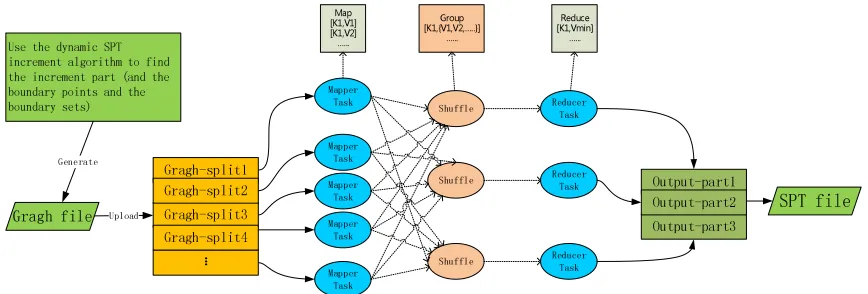
node and use TaskTraker of HADOOP to complete the mapper task. The mapper task mainly generates and calculates the weights of each path between a vertex and the source vertex. Then, reducer task will select the shortest path between the vertex and the source vertex. Finally Integrate these reduce results together. The overall process is shown in figure 1.

Gragh file Upload

Mapper Task

Mapper Task

Mapper Task

Gragh-split1

Gragh-split3 Gragh-split2

Gragh-split4 ...

Mapper Task

Mapper Task

Map [K1,V1] [K1,V2]

…...

Shuffle

Shuffle

Shuffle

Group [K1,{V1,V2,…..}]

…...

Reducer Task

Reducer Task

Reducer Task

Reduce [K1,Vmin]

…...

Output-part1

Output-part3

Output-part2 SPT file

Use the dynamic SPT increment algorithm to find the increment part (and the boundary points and the boundary sets)

Generate

Figure 1. The overall process.

The following is a detailed description of the algorithm:

1. Using the dynamic SPT increment algorithm[4,5,6,7] to find out the incremental part.

The incremental part includes the boundary vertices and the related edges between them. By using the dynamic SPT increment algorithm, find out the boundary vertices then regenerate the SPT path of the incremental part.

The definition of boundary points is as a set between source vertex and vertices (or the adjacent of the vertices) which are on the shortest path when some edge values on the weighted directed graph change. The Boundary points are vertices which make the original SPT tree change, these Boundary points can be called the boundary vertices.

Take Figure 2 as an example, the solid line is the original SPT tree. When the Weight (A→C) changed from 4 to 1, and the change edge is on SPT tree. Although the C vertex is still in the SPT tree, the adjacent vertex E of the C, which is not in the SPT tree originally, may now become a vertex in the SPT tree. Clearly, E is the boundary vertex. Therefore, the weighted boundary directed graph formed by the boundary vertices and the edges related to boundary vertices, will be used as the incremental part to regenerate the SPT path.

1

6

Figure 2.Boundary vertices definition.

2. Convert the incremental partially weighted directed graph into the input file Graph.

V1 V2

V3 V4

V5

V6 1

1 2

V1 0 V2:2|V3:4 NULL V2 100000 V3:3|V4:1|V5:1 NULL V3 100000 V4:1| V6:1 NULL V4 100000 V5:1 NULL V5 100000 V6:1 NULL V6 100000 NULL NULL

Figure 3.Weighted directed graph G.

Each line of content in the file is explained in detail below. In the first line, the first column of the first line is the vertex name of the current vertex. The second column is the shortest path value for the current vertex. Namely, the value is the minimum value between all reachable paths that currently traversed. The vertex V1 is the source vertex in this figure, so the value is 0, the initial value of the shortest distance of other vertexes is 100000 (representing unreachable). The third column is the adjacency list of the current vertex, for example, the V2:2|V3:4 in the first line represents the vertex V1 has two adjacent vertices, i.e., vertex V2 and vertex V3, and the weight of the two edges is Weight (V1→V2) =2, and Weight (V1→V3) =4. The fourth column represents the parent vertex of the current vertex in the SPT tree, which have not been traversed in the initial input file, so the value of all vertices here are initial value "NULL".

Each line of data can be described as

Vertex Distance(Vertex) Adj(Vertex:Value) P(Vertex) (1) 3. Implement the Map () function.

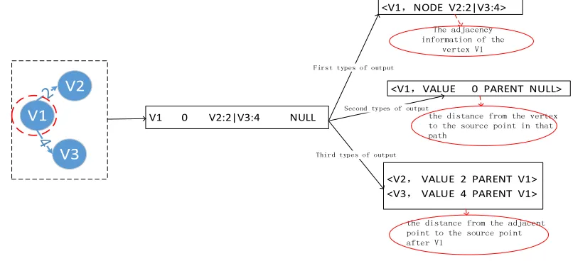
In this algorithm, the Map function has two output formats and three output paths. In two output formats, one represents the adjacency list of vertexes, while the other is used to represent the shortest path. To distinguish these two formats, the determinant "NODE" and "VALUE" are introduced. The output with "NODE" indicates that the output is the adjacency list of the current vertex, while the output with "VALUE" represents the output is the shortest path information of the current vertex. Here is an example of vertex V1 in Figure 3:

V1 V2

V3

V1 0 V2:2|V3:4 NULL

<V1，NODE V2:2|V3:4>

<V1，VALUE 0 PARENT NULL>

<V2， VALUE 2 PARENT V1> <V3_， VALUE 4 PARENT V1> First types of output

Second types of output

Third types of output

The adjacency information of the

vertex V1

the distance from the vertex to the source point in that path

the distance from the adjacent point to the source point after V1

Figure 4.Map output with vertex V1 as the example.

1) The first output path is < current vertex, the adjacency list of the current vertex >, and the symbol is:

<Vertex, NODE Adj(Vertex:Value)> (2) Take the first line of Figure 3 Graph file as an example, the output is <V1, NODE V2:2|V3:4>, as shown in Figure 4, the first output.

<Vertex, VALUE Distance(Vertex) PARENT P(Vertex)> (3) Take the first line of Graph file as an example, the output is <V1, VALUE 0, PARENT, NULL>, as shown in Figure 4, the second output.

3) The third output path is < adjacency vertex, the distance of the adjacent vertex to the source vertex through the current vertex and the parent vertex of the adjacent vertex >.

Correspond to the MapReduce, the key is the vertex in adjacency list of the current vertex, i.e., key= Vertex’, Vertex’∈Adj(Vertex). The value is the shortest path of adjacency vertex Vertex’: Distance (V ') = Distance (Vertex) + W (Vertex = Vertex) when the shortest path goes through the edge Vertex→Vertex'. Therefore, symbols are represented as:

< Vertex’, VALUE Distance(Vertex’) PARENT Vertex>,Vertex’∈ Adj(Vertex) (4) Take the first line of Graph file as an example, the output is:

<V2, VALUE 2 PARENT V1> , <V3, VALUE 4 PARENT V1> As shown in Figure 4, the third output.

Take Figure 3 as an example, the output of the Map task is as Figure 5:

<V1，，，，NODE V2:2|V3:4> <V1，，，，VALUE 0 PARENT NULL> <V2，，，，VALUE 2 PARENT V1> <V3，，，，VALUE 4 PARENT V1> <V2，，，，NODE V3:3|V4:1|V5:1> <V2，，，，VALUE 100000 PARENT NULL> <V3，，，，VALUE 5 PARENT V2> <V4，，，，VALUE 3 PARENT V2> <V5，，，，VALUE 3 PARENT V2>

<V3，，，，NODE V4:1|V6:1>

<V3，，，，VALUE 100000 PARENT NULL> <V4，，，，VALUE 100001 PARENT V3> <V6，，，，VALUE 100001 PARENT V3> <V4，，，，NODE V5:1>

<V4，，，，VALUE 100000 PARENT NULL> <V5，，，，VALUE 100001 PARENT V4>

<V5，，，，NODE V6:1>

<V5，，，，VALUE100000 PARENT NULL> <V6，，，，VALUE 100001 PARENT V5> <V6，，，，NODE NULL>

<V6，，，，VALUE100000 PARENT NULL>

The Map task output of Node1 The Map task output of Node2 The Map task output of Node3

Figure 5. Map output with vertex V1 as the example.

4. By shuffling[8] on the mapper results, obtain each key corresponding to its reduce machine node. This part is implemented by the MapReduce framework, and the role of shuffle is According to the machine nodes number and the key to determine the current output data should be handed over to which reduce task to reduce. The default is to hash key and then modulo on the number of reduce tasks.

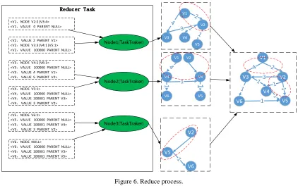
5. Implement Reduce function and obtain output results.

For value with "NODE" tags, the values do not need to be processed because there is no change in the structure of the digraph, assign the value after "NODE" tag directly to the variable Adjacency needed to output.

For the value with the "VALUE" tag, representing the shortest path information, therefore, the shortest path value is selected for Min. The value after "VALUE" tag is taken as the shortest distance of the current vertex, and the tag after "PARENT" is used as the parent vertex of the current vertex in the shortest path tree, that is

Distance(key) = Min.value , P(key) = Min.parent (5) Therefore, the output value of the Reduce function is < the current vertex, the shortest distance value of the current vertex, the adjacency vertex of the current vertex, the parent vertex of the current vertex in SPT >, represented by symbols as:

<V1，NODE V2:2|V3:4> <V1，VALUE 0 PARENT NULL>

<V2， VALUE 2 PARENT V1> <V2，NODE V3:3|V4:1|V5:1> <V2，VALUE 100000 PARENT NULL>

<V3，NODE V4:1|V6:1> <V3，VALUE 100000 PARENT NULL> <V3， VALUE 4 PARENT V1> <V3， VALUE 5 PARENT V2>

<V4，NODE V5:1>

<V4，VALUE 100000 PARENT NULL> <V4， VALUE 100001 PARENT V3> <V4， VALUE 3 PARENT V2>

<V5，NODE V6:1>

<V5，VALUE 100000 PARENT NULL> <V5， VALUE 100001 PARENT V4> <V5， VALUE 3 PARENT V2>

<V6，NODE NULL>

<V6，VALUE 100000 PARENT NULL> <V6， VALUE 100001 PARENT V3> <V6， VALUE 100001 PARENT V5>

Node1(TaskTraker)

Node2(TaskTraker)

Node3(TaskTraker)

V3 V4

1

V5 V6

V2

V6 V5

Reducer Task Reducer TaskReducer Task Reducer Task

V1

V2 V3

V4

V5

V1

V2

V3 V4 V5

1

V1 V2

3

V6

Figure 6.Reduce process.

Take Figure 3 as an example, the output of Reduce is shown in table 1:

Table 1. The output of Reduce V1 0 V2:2|V3:4 NULL V2 2 V3:3|V4:1|V5:1 V1 V3 4 V4:1|V6:1 V1 V4 3 V5:1 V2 V5 3 V6:1 V2 V6 100000 NULL NULL

6. Repeat iterations until the shortest path tree is generated.

From the output of the Reduce function, it can be seen that the result obtained after the execution of the MapReduce Job is not the final shortest path tree. Some of the vertices have not yet been traversed, and the traversed shortest path is not really the shortest path. Because of the output file produced by MapReduce Job is completely in agreement with the input file in format, and the output file is also stored on the distributed file system HDFS. Therefore, the output file can be as the input file for the next round of MapReduce Job, and iterate through the 2-4 step until the shortest path tree is generated.

Take Figure 3 as an example, the final reduce result file and the resulting shortest path tree is shown in Figure 7:

V1

V2 V3

V4 V5

V6

V1 0 V2:2|V3:4 NULL

V2 2 V3:3|V4:1|V5:1 V1

V3 4 V4:1|V6:1 V1

V4 3 V5:1 V2 V5 3 V6:1 V2 V6 5 NULL V3

Table 2. Integral code flow.

function (map)

for each input sentence: split into three types outputs:

{Vertex, NODE Adj(Vertex)} {Vertex, VALUE Distance(Vertex) PARENT P(Vertex)}

{Vertex’, VALUE

Distance(Vertex’) PARENT Vertex [Vertex’∈ Adj(Vertex), Distance(Vertex’) =

Distance(Vertex) + W(Vertex→V’)]}

function (reduce)

if label contains ‘VALUE’ Distance(key) = Min.value P(key) = Min.parent if label contains ‘NODE’

get Adj(Vertex) output:

{Vertex Distance(Vertex) Adj(Vertex:Value) P(Vertex)} end function

end function

Experimental Results and Evaluation

This paper studies and implements the dynamic SPT increment algorithm for aircraft booking based

on Hadoop distributed platform. The dynamic SPT increment algorithm[9,10] is good at solving the

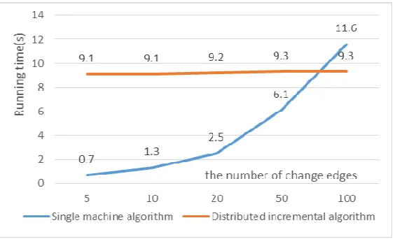
situation that the number of boundary vertices is not too many. When the number of boundary vertices in SPT is increased to a larger amount, the performance of the algorithm is limited, While the dynamic SPT increment algorithm based on Hadoop can deal with large-scale changes of the edge weights and vertices in the directed weighted graphs, the performance of this algorithm depends on the number of machine nodes participating in the computation.

Using the real data as input, control the number of change edges respectively as 5, 10, 20, 50, 100, test the two algorithms, the test results are shown in Figure 8:

Figure 8. Comparison of algorithm test results.

Summary

Based on the special needs of China United Airlines, by using its information of the air route network, this paper proposes a dynamic SPT increment algorithm for aircraft booking based on Hadoop. The experiment was carried out by the aerial route map provided by China United Airlines. The experimental results showed that the algorithm has good practical effects. Because of the complexity, and variety of the aviation system in reality, the system uses the characteristics of distributed computing on the Hadoop platform to complete the calculation of large amount of data, and effectively improves the efficiency of the system.

Acknowledgement

This work is supported by National Natural Science Foundation of China under Grant No.61702043 and Fundamental Research Funds for the Central Universities under Grant No.500417062.

References

[1] Bin Xiao, Jiannong Cao, Qin Lu. Dynamic SPT update for multiple link state decrements in network routing[J]. The Journal of Supercomputing, 2008: 463-464.

[2] Zhang Xiaohong, Zhong Zhiyong, Feng Shengzhong, et al. Improving data locality of MapReduce by scheduling in homogeneous computing environments [C] //Parallel and Distributed Processing with Applications (ISPA), 2011 IEEE 9th International Symposium on. 2011:120-126.

[3] E. W. Dijkstra. A Note on Two Problems in Connection with Graphs. Numerical Math., vol. 1, pp. 269-271, 1959.

[4] G. Ramalingam, T.W. Reps. An Incremental Algorithm for a Generalization of the Shortest-Path Problem. J. Algorithms. Vol. 21. No. 2. pp. 267-305, 1996.

[5] Xiao B, Zhuge Q, Sha EH-M (2004) Efficient algorithms for dynamic update of shortest path tree in networking. J Comput Appl 11:60–75.

[6] Xiao B, Cao J, Zhuge Q, Shao Z, Sha EH-M (2004) Shortest path tree update for multiple link state decrements. In: Proceedings of the IEEE global telecommunications conference (Globecom 2004), pp. 1163–1167.

[7] Zhang B, Mouftah HT (2002) A destination-driven shortest path tree algorithm. In: Proceedings

of the IEEE international conference on communications, April 2002, vol 4, pp 2258–2262.

[8] Puneet Agarwal, Gautam Shroff, Pankaj Malhotra. Approximate Incremental Big-Data Harmonization[A]. //2013 IEEE International Congress on Big Data[C], Santa Clara: IEEE, 2013: 131-134.

[9] Sebastien Felix, Jerome Galtier. Shortest Paths and Probabilities on Time-Dependent Graphs - Applications to Transport Networks[A]. //2011 11th International Conference on ITS Telecommunications[C], St. Petersburg: IEEE, 2011:152-160.