A COMPUTATIONALLY EFFICIENT PROCEDURE FOR
DATA ENVELOPMENT ANALYSIS
Srinivasan Parthasarathy
Operational Research Group, Department o f Management London School of Economics and Political Science
Thesis submitted to the London School of Economics and Political Science, for the degree o f Doctor of Philosophy
UMI Number: U 615720
All rights reserved
INFORMATION TO ALL U SE R S
The quality of this reproduction is d ep en d en t upon the quality of the copy subm itted.
In the unlikely even t that the author did not sen d a com plete m anuscript
and there are m issing p a g e s, th e se will be noted. Also, if material had to be rem oved, a note will indicate the deletion.
Dissertation Publishing
UMI U 615720
Published by ProQ uest LLC 2014. Copyright in the Dissertation held by the Author. Microform Edition © ProQ uest LLC.
All rights reserved. This work is protected against unauthorized copying under Title 17, United S ta tes C ode.
ProQ uest LLC
789 East E isenhow er Parkway P.O. Box 1346
TW5S&?
F
The author hereby declares that the work presented in this thesis is his own.
ABSTRACT
This thesis is the final outcome of a project carried out for the UK’s Department for Education and Skills (DfES). They were interested in finding a fast algorithm for solving a Data Envelopment Analysis (DEA) model to compare the relative efficiency o f 13216 primary schools in England based on 9 input-output factors. The standard approach for solving a DEA model comparing
n units (such as primary schools) based on m factors, requires solving 2n linear programming (LP) problems, each with m constraints and at least n variables. At m = 9 and n = 13216, it was proving to be difficult.
The research reported in this thesis describes both theoretical and practical contributions to achieving faster computational performance. First we establish that in analysing any unit t only against some critically important units - we call them generators - we can either (a) complete its efficiency analysis, or (b) find a new generator. This is an important contribution to the theory of solution procedures of DEA. It leads to our new Generator Based Algorithm (GBA) which solves only n LPs of maximum size (im x k), where k is the number of generators. As k is a small percentage o f n, GBA significantly improves computational performance in large datasets. Further, GBA is capable o f solving all the commonly used DEA models including important extensions of the basic models such as weight restricted models.
In broad outline, the thesis describes four themes. First, it provides a comprehensive critical review o f the extant literature on the computational aspects of DEA.
Second, the thesis introduces the new computationally efficient algorithm GBA. It solves the practical problem in 105 seconds. The commercial software used by the DfES, at best, took more than an hour and often took 3 to 5 hours making it impractical for model development work.
experiments. It is also shown that GBA is consistently better than BuildHull and is a viable tool for solving large scale DEA problems.
ACKNOWLEDGEMENTS
I recall Professor Abraham Chames’ advice to aspiring PhD students to choose the teacher and not the topic. Even though I got to hear about this recently, I am glad that I followed it. I started my PhD with absolutely no knowledge on the topic but had the trust that I chose my teacher well. I am indebted to my supervisor, Professor Gautam Appa for giving me the opportunity to study for a PhD under his supervision with financial support. I am also indebted to him for his unfailing academic rigour and continuous encouragement. I cannot fail to mention his patience and attentive attitude towards me all these years for I tested him to his extreme emotions on numerous occasions. He was and remains a pillar in my life.
I am deeply indebted to Dr. Susan Powell for helping me with my writing style and for her attention to detail. I owe much to her patience and guidance in shaping this thesis.
I am also indebted to Professors Rajiv Banker and Ram Natarajan for inviting me to collaborate with them during my PhD study.
I am grateful to Professors Jose Dula and Emmanuel Thanassoulis for their patience and assistance with many o f my persistent queries on various theoretical aspects of DEA.
I am grateful to Professor Ailsa Land for her feedback on the computational aspects of my thesis and to Mr. George Mitchell on the preface.
I would like to thank the OR department manager Brenda Mowlam, and the administrators Jenny Robinson, Richard Szadura and Lucy Underhill for their patience and help with all sorts o f administrative requests over the years.
For their continued patience, help and friendship, I thank my fellow PhD students, Ionna Katrantzi, Kostas Papalamprou, Nikos Argyris, Nayat Horzoglou, Anastasia Kouvela, Dimitrios Karamanis, Kai Becker, Shweta Agarwal, Ana Barcus and Sumithra Sribashyam.
Thanks are due to my friends over many years - Cristiana, Anupama, Ernie, Leong, Lena, Emily, Diana, Aijen, Ofer, Joelle, Lida, Maha and many more - for making my life much more pleasant in many ways.
DEDICATION
PREFACE
I Motivation and Genesis
The issue addressed in the work recorded in this thesis is the computational efficiency in applying Data Envelopment Analysis (DEA) and how this may be improved.
In 2005, the Value for Money (VfM) unit of the Department for Education and Skills (DfES)1 commissioned my supervisor, Professor Gautam Appa, to develop procedures for speeding up computation o f DEA models for large scale datasets. The DfES had decided to use DEA to identify the well-run primary schools in England and to provide benchmarks based on these for the poorly-run ones. DEA divides the units (primary schools in this case) under investigation into efficient and not efficient and finds peers amongst the efficient ones which are relevant for setting targets for the inefficient ones. So in some sense DEA was suitable for their purpose. However, in carrying out DEA computations they encountered one big difficulty. The performance analysis software they were using for processing DEA datasets, PIM DEASoft-v2 (http://www.deasoftware.co.ukA. took too long to solve datasets with more than 5000 units and sometimes required multiple attempts to run them to completion. Professor Appa was given a grant to appoint a PhD student to review current computational methods and come up with improved ones. In September 2005, he drafted me as his PhD student and it was agreed that under grant EOR/SBU/2003/208 from the DfES, my research would review the extant literature on the different solution procedures to process DEA datasets and develop new techniques to realize improved computational efficiency.
It is worth noting that although the issues discussed in this thesis arose in connection with comparing the performance of primary schools, they could equally have arisen in many other contexts which involve large datasets (for example, in comparing the performance o f branches of a bank, in financial
applications such as portfolio analysis etc.). The methods developed herein therefore can be expected to have wide applications.
It is also important to note that there are certain applications in DEA that necessitate solving multiple DEA LPs for each unit and are computationally intensive even for medium scale datasets. These include the bootstrapping
technique developed in Simar and Wilson (1998) and Simar and Wilson (2000),
outlier identification technique developed in Wilson (1993), Kuosmanen and
Post (1999), Simar (2003) and Banker and Chang (2006), various methods to estimate the returns to scale of units in DEA developed in Banker and Thrall (1992), Fare and Grosskopf (1994) and Banker et al (2004), and methods to estimate the productivity growth using the malmquist productivity analysis
technique developed in Fare et al (1994), Ray and Desli (1997), Simar and Wilson (1999) and Banker et al (2010). The algorithm developed in this thesis is also expected to come useful in reducing the computational work in such intensive applications.
II Foundation and Development
Upon reviewing the literature on the computational aspects o f DEA, only three strands of relevant research were identified. These (discussed in detail in Chapter 3) comprised of:
1. the DEA based pre-processing ideas o f Ali (in Ali (1993) and Chen and Ali (2002)),
2. the hierarchical decomposition algorithm o f Barr and Durchholz (1997), and
3. the BuildHull algorithm of Dula (1998).
came up with one that kept the main feature o f BuildHull but cut down the number of LPs to be solved by half.
To evaluate any unit in DEA, it is sufficient to have data on its relevant peers from the dataset. Hence, comparing an unit with all the units in the dataset is unnecessary. This is especially important when a vast majority of units are inefficient and hence well known to have no relevance in the evaluation of any other unit. Most real life datasets have this feature. For example, the number of relevant efficient units in the primary school data was only 188 out of 13,216. We will call the relevant efficient units generators for now and define the term precisely later. The main strength of BuildHull comes from the fact that it identifies all the generators in a first pass where each unit is tested against already identified generators to see if it is inefficient in comparison. If it is, it can be discarded; if not, BuildHull has a way to find some hitherto undiscovered generator. So it requires n LPs to find all the generators (e.g., 188 schools) in a dataset and no LP will have more than k + l units in it if there are k generators (here, 188 schools). For the primary schools problem, BuildHull will solve 13216 LPs with no more than 189 variables in each LP in the first phase. In phase 2, BuildHull will solve one LP for each unit which is not a generator, with only the
k generators and the unit itself in each LP; so 13028 LPs with 189 variables in each.
The improvement we make is to find a way to work only with known generators but in such a way that at each step we either finish the analysis of unit
t under investigation or find a new generator, thus needing to solve only n LPs with no more than k variables at any step. The main tool for achieving this is the use of super-efficiency model of DEA (introduced in Andersen and Petersen (1993)) and a ratio test to find a new generator.
In the first instance we were able to deal with these finer points by assuming them away. So we assumed that the data entries were all positive, which took care o f both the infeasibility and the indeterminate ratio problems. And ties were waved aside by assuming that there was a way to solve them. But eventually we had to solve these problems head on. It was found that indeterminate ratios were only problematic when there were ties and so can be handled by our tie breaking procedure. Fortunately we were able to find a closed form solution to the problem of breaking ties. It turns out that the same closed- form solution can also be used to find strictly positive optimal weights for all the factors for each generator.
Ill Organization of the thesis
Chapter 1 starts with an introduction to the DEA technique familiarising the reader with some of the important concepts by means o f a graphical illustration, followed by a systematic investigation. We then give a brief history o f the evolution of DEA.
Chapter 2 presents the standard DEA LP models, viz., constant and variable returns to scale models under input and output orientation and additive models, used in DEA applications. The chapter also provides a brief critical review o f an important variant of these, namely, the super-efficiency models, which we employ in the construction o f our new algorithm developed in chapter 4.
To reduce the computational strain in processing DEA datasets, various heuristics and alternative efficient algorithms have been developed in the literature over the years. Chapter 3 presents a comprehensive critical review of these, identifying the three main strands mentioned earlier.
for Dula’s BuildHull algorithm. In contrast to BuildHull, our algorithm avoids solving a second LP for the 8 DMUs.
Chapter 5 addresses the technical challenges in using GBA for general (not necessarily positive) datasets for all the standard DEA models described in chapter 2. For each specific DEA model, we present conditions under which the two main technical challenges o f infeasibility and indeterminate ratios can or cannot occur when applying GBA.
The purpose o f chapter 6 is to present ways to handle the technical challenge o f infeasibility. We examine two different approaches to handle it, viz., clustering and penalty. Within the penalty method, we examine two different techniques, viz., employing a big penalty and a small penalty. The clustering technique works under restrictive conditions while the penalty methods can tackle infeasibility under all circumstances.
In chapter 7, we examine ways to deal with the remaining technical difficulties o f GBA. We first show that within GBA the problem of indeterminate ratios is only relevant when there is a tie in the rule for finding a new generator. Then we provide novel closed-form solutions to resolve ties. Finally we extend these closed-form solutions to construct a strictly positive set of multiplier values for the generators.
Chapter 8 presents the computational results of processing datasets using various DEA models. While doing so, we compare the computational performance o f GBA against BuildHull and the conventional solution procedure. For VRS models we compare the computational performance o f GBA against the other two using the problem suite that Dula (1998, 2008, 2010) employed in his studies. As Dula does not provide any comparisons for CRS models we use a problem suite developed for this purpose. As the main contender for GBA is BuildHull, we give separate diagrams comparing just these two.
GLOSSARY OF THE TERMS AND SYMBOLS
DMU - Decision Making Unit.
(DMUs denote the plural form o f DMU and not the s* DMU) Units - Refers to DMUs.
PPS - Production Possibility Set. RTS - Returns to Scale.
CRS - Constant Returns to Scale. VRS - Variable Returns to Scale.
n - Number o f observed decision making units.
ml - Number of input factors in the dataset.
m2 - Number of output factors in the dataset.
(X , Y), ( x , Y), [ x , Y) - Activity o f an unit with support over R +n)2.
X - Input component (vector) of the activity (X, Y) with support overR ”1.
Y - Output component (vector) of the activity (X , Y) with support overR™2.
[ x j ,Yj)~ Activity of an observed unit j.
( X t ,Yt ) - Activity of an observed unit (DMUt) that is currently being evaluated.
X - Matrix o f inputs of all the observed units of size m ^ n .
Y - Matrix o f outputs o f all the observed units o f size m2x n . A,j or jLLj - Intensity variable of an observed unit j.
s' - Input slack vector with support o verR ”1.
s ° -Output slack vector with support over R™2.
v - Input weight vector with support overR™1.
u - Output weight vector with support overR™2.
6 - Variable that depicts the input efficiency of DMUt.
(f) - Variable that depicts the output inefficiency of DMUt.
0 - Zero vector with dimension decided by the context.
Density -Percentage of extreme-efficient units in a DEA exercise. P-K efficient - Pareto-Koopmans efficient.
GBA - Generator Based Algorithm. LP - Linear Programming.
MILP - Mixed Integer Linear Programming. DGP - Data Generating Process.
CONTENTS
ABSTRACT...3
ACKNOWLEDGEMENTS...5
DEDICATION...7
PREFACE...8
I Motivation and Genesis... 8
II Foundation and Development...9
III Organization of the thesis... 11
GLOSSARY OF THE TERMS AND SYMBOLS... 13
CONTENTS...15
LIST OF TABLES...21
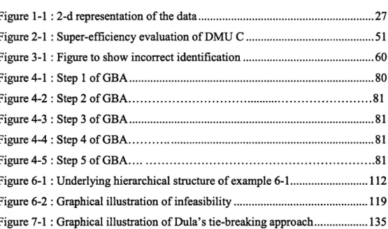
LIST OF FIGURES...23
LIST OF CHARTS...24
LIST OF APPENDICES...25
1 INTRODUCTION TO DATA ENVELOPMENT ANALYSIS... 26
1.1 Background...26
1.2 Theoretical Framework... 31
1.2.1 Production Possibility Set under the Constant Returns to Scale... 32
1.2.2 Production Possibility Set under the Variable Returns to Scale... 33
1.2.3 Definitions and Measures o f Technical Efficiency...34
1.3... Concepts of Efficiency...36
1.4 A brief history o f the evolution o f D E A ...38
2 LINEAR PROGRAMMING MODELS USED IN DEA... 40
2.1 LP models under Constant Returns to Scale assumption...41
2.2 LP models under Variable Returns to Scale assumption...44
2.3 Additive models under CRS and VRS assumptions...46
2.4 Introduction to Super-Efficiency model...48
2.4.1 Linear Programs employed in super-efficiency models...48
2.4.2 An illustration of the super-efficiency m odel... 50
2.4.3 A brief literature review on super-efficiency m odels...52
2.5 Conclusion... 54
3 COMPUTATIONAL ISSUES IN SOLVING DEA MODELS - A CRITICAL LITERATURE REVIEW ...55
3.1 Ali’s contributions: pre-processing and LP acceleration techniques... 57
3.1.1 Limitations of Ali (1993), and Chen and Ali (2002)...60
3.2 Barr and Durchholz (1997) contribution: Hierarchical Decomposition procedure...63
3.3 Dula’s BuildHull algorithm... 65
3.4 Algorithmic characteristics of competing solution procedures... 67
3.5 Conclusion... 69
4 GENERATOR BASED ALGORITHM FOR SOLVING THE INPUT-ORIENTED CRS MODEL... 70
4.1 Background and definitions... 70
4.2 Modified input-oriented CRS super-efficiency model...72
4.3.1 Ratio Rj... 73
4.3.2 Procedure FindNewGen... 76
4.3.3 Description of G B A ...78
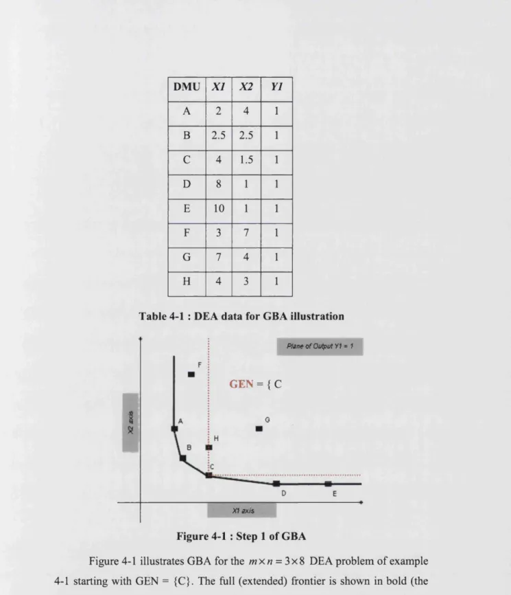
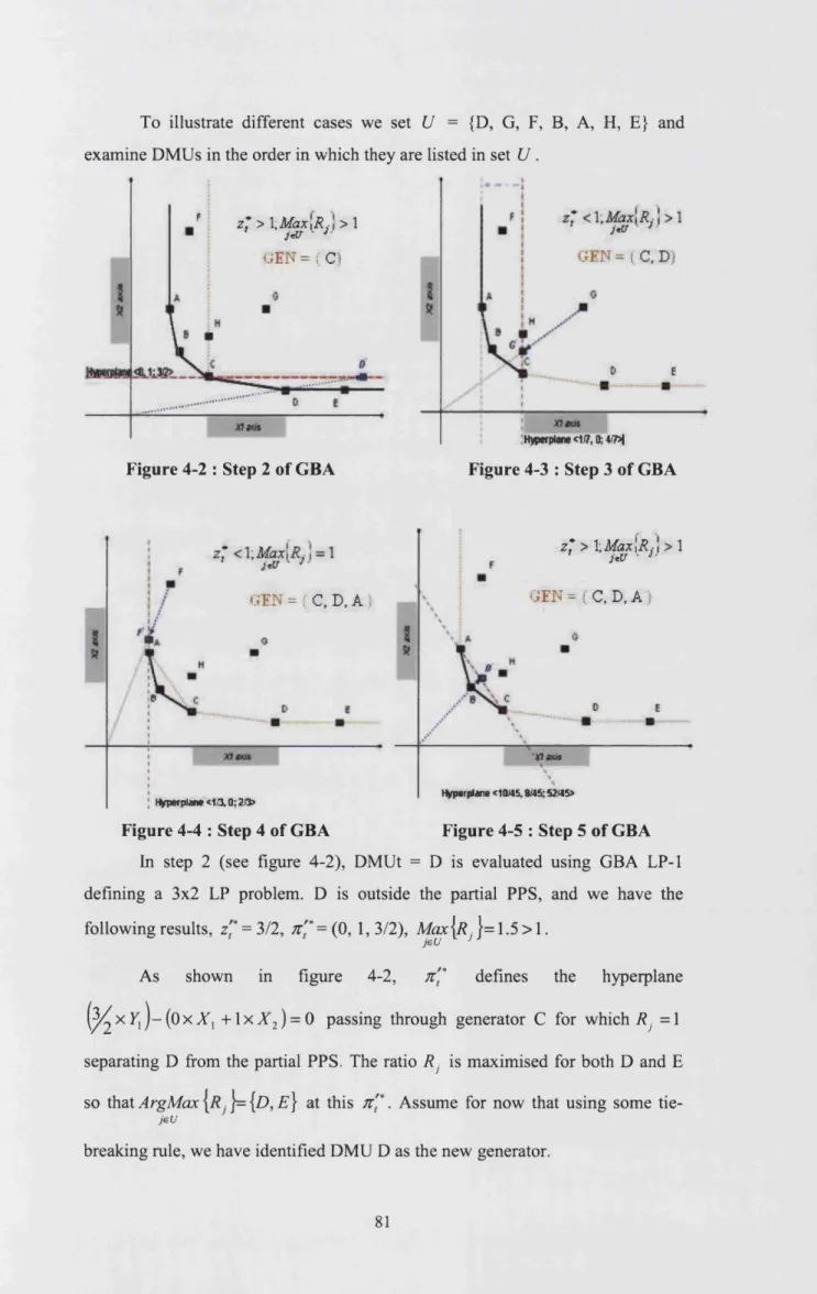
4.4 An illustration of GBA...79
4.5 Ratios and Reduced cost values... 83
4.6 Advantages of GBA...84
4.6 Conclusion... 85
5 TECHNICAL CHALLENGES AND EXTENSION OF GBA TO OTHER DEA MODELS...86
5.1 GBA for the general input-oriented CRS model...87
5.1.1 LP infeasibility... 87
5.1.2 Indeterminate ratios...89
5.2 GBA for the output-oriented CRS model... 90
5.2.1 LP infeasibility...91
5.2.2 Indeterminate ratios...91
5.3 GBA for the input-oriented VRS m odel...93
5.3.1 Using the reduced costs RCj instead of the Rj values in GBA 95 5.3.2 LP infeasibility...97
5.3.3 Indeterminate ratios...98
5.4 GBA for the output-oriented VRS m odel...99
5.4.1 Infeasibility... 101
5.4.2 Indeterminate ratios...101
5.5.1 Infeasibility...104
5.5.2 Indeterminate ratios... 105
5.6 GBA for solving the VRS additive m odel...105
5.6.1 Infeasibility...107
5.6.2 Indeterminate ratios... 107
5.7 Conclusion... 108
6 WAYS TO RESOLVE THE LP INFEASIBILITY ISSUE IN GBA...109
6.1 Infeasibility in the input-oriented CRS m odel... 109
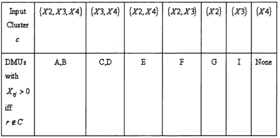
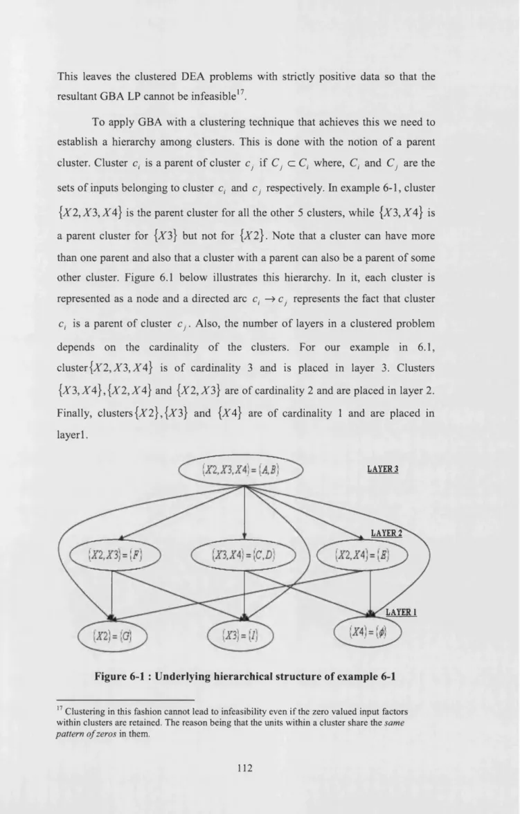
6.1.1 Natural Clustering for the input oriented CRS case...109
6.1.1.1 Pros and Cons of the Clustering technique... 116
6.1.2 Penalty methods for the input oriented CRS case...117
6.1.2.1 Big Penalty or Big-M method...117
6.1.2.2 Small-m method... 123
6.2 Infeasibility in the input-oriented VRS model... 124
6.2.1 Big-M method...124
6.2.2 Small-m method...125
6.3 Infeasibility in the output-oriented VRS model... 126
6.4 Infeasibility in the CRS and VRS additive models... 128
6.5 Conclusion... 129
7 CLOSED-FORM SOLUTIONS TO RESOLVE TIES AND CONSTRUCT NON-ZERO MULTIPLIER VALUES... 130
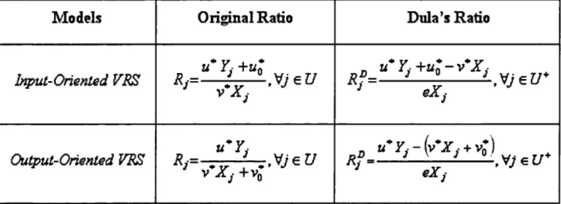
7.1.1 Dula’s ratio...130
7.1.2 Indeterminate ratios and their association with tied ratios... 132
7.2 Ways to resolve tie s ...133
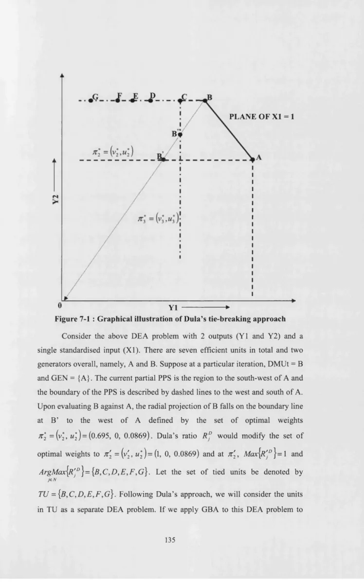
7.2.1 Dula’s approach to resolve ties...134
7.2.2 Closed-form solutions to resolve ties...136
7.2.2.1 Closed-form solution to resolve ties under V R S ...138
1 .2 2 2 Closed-form solution to resolve ties under CRS...143
7.3 Strictly Positive multiplier values for generators... 152
7.3.1 Literature review...152
7.3.2 A closed-form solution for achieving positive weights under CRS... 155
7.3.2.1 Illustration of the closed-form solution to ensure positive weights under CRS... 158
7.3.3 Closed-form solution for achieving positive multiplier values under VRS... 161
7.3.3.1 Illustration of the closed-form solution to ensure positive weights under V R S ... 163
7.4 Conclusion... 165
8 COMPUTATIONAL RESULTS FOR GBA...167
8.1 Competitive algorithms to solve the output-oriented VRS model...168
8.1.1 Description of the problem suite...168
8.1.2 Technology and Implementations...169
8.1.2.2 Description o f BuildHull and the Standard two-phase
algorithm... 173 8.1.3 Limitations of the computational experiments... 175 8.1.4 Computational results and comparison of algorithmic
performances...177 8.2 Competitive algorithms to solve the additive VRS model...186 8.2.1 Comparison of algorithmic performances... 186 8.3 Competitive algorithms to solve the input-oriented CRS model... 189 8.3.1 Problem suite under CRS... 189 8.3.2 Description of G B A ... 191 8.3.3 Description o f BuildHull and standard algorithm...193 8.3.4 Limitations o f the computational experiments...195 8.3.5 Computational results and comparison of algorithmic
performances... 195 8.4 Conclusion... 205
9 DIRECTIONS FOR FUTURE RESEARCH... 206
9.1 Enhancing the computational experiments...206 9.2 Extension of GBA to handle negative data and the FDH models...207 9.3 Extension of the closed-form solutions...209
LIST OF TABLES
LIST OF FIGURES
LIST OF CHARTS
LIST OF APPENDICES
Appendix 1 - Shephard’s (1970) output distance function and related Debreu-Farrell measure... 210 Appendix 2 - July 2006 report to the DfE on Dula’s w ork...212 Appendix 3 - Proof that Xt is either 0 or 1 in the penalty enabled GBA models ...233 Appendix 4 - R codes to solve the output-oriented VRS model using GBA, BuildHull and the standard DEA algorithm...235 Appendix 5 - Computational performance o f the competitive algorithms in solving the output-oriented VRS m odel...247 Appendix 6 - R codes to solve the additive VRS model using GBA, BuildHull and the standard DEA algorithm... 249 Appendix 7 - Computational performance o f the competitive algorithms in solving the additive VRS model... 259 Appendix 8 - R codes o f the two alternative GBA approaches and an alternative BuildHull approach to solve the additive VRS m odel... 261 Appendix 9 - R codes o f the DGP, and GBA, BuildHull and the standard DEA algorithm to solve the input-oriented CRS model... 275 Appendix 10 - Computational performance of the competitive algorithms in solving the input-oriented CRS m odel... 287 Appendix 11 - R code to solve the output-oriented VRS model with built-in
1 INTRODUCTION TO DATA ENVELOPMENT ANALYSIS
1.1 Background
Data Envelopment Analysis (DEA) is a linear programming (LP) based technique that is used to determine the relative efficiency o f homogeneous operating units responsible for converting inputs to outputs. The operating units, labelled in the DEA literature as Decision Making Units or DMUs, are similar in that they employ the same type o f inputs to produce the same type of outputs. Conventionally, the purpose o f a DEA exercise is to find the relative efficiency by which a DMU transforms its inputs to outputs when compared to other similar units. Relative efficiency, being a dimensionless scalar, does not require the various inputs and outputs to be measured in the same unit of measurement.
DEA is a non-parametric method in the sense that a functional form relating the inputs and outputs need not be specified apriori. It is also a frontier based method in that all the units are compared to the best practice units which also consume the same set o f inputs to produce the same set of outputs.
Before we get into the theoretical framework o f DEA, we will familiarise ourselves with some of the important concepts in DEA using a simple example. For ease of discussion, we will examine these concepts rather loosely and consign a rigorous treatise o f them to section 1.2. Consider the following two inputs (XI and X2), one output (77), 9 DMU example portrayed in figure 1-1. The data for the example is provided in table 1-1.
DMU X I X2 Y1
A 2 9 1
B 4 6 1
C 6 3.5 1
D 10 2.5 1
E 12 2.5 1
F 2.5 13 1
G 9 5 1
H 5 6.5 1
I 8 3 1
FLAJNTE OF Y1 = 1
X2
,'H ’
XI
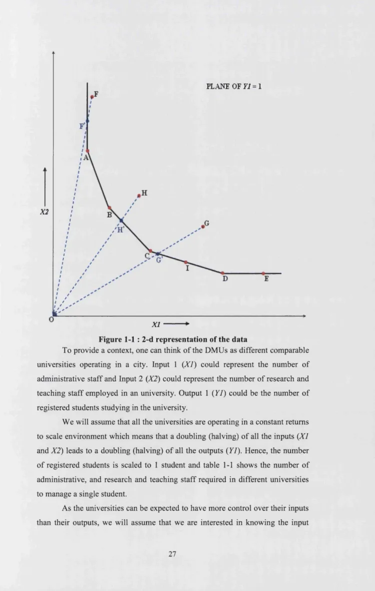
Figure 1-1 : 2-d representation of the data
To provide a context, one can think o f the DMUs as different comparable universities operating in a city. Input 1 (XI) could represent the number of administrative staff and Input 2 (X2) could represent the number o f research and teaching staff employed in an university. Output 1 (17) could be the number o f registered students studying in the university.
We will assume that all the universities are operating in a constant returns to scale environment which means that a doubling (halving) o f all the inputs (XI and X2) leads to a doubling (halving) of all the outputs (Yl). Hence, the number o f registered students is scaled to 1 student and table 1-1 shows the number of administrative, and research and teaching staff required in different universities to manage a single student.
efficiency o f these universities. This means that we are interested in knowing the minimum proportion of an university’s current input usage that is sufficient, in comparison with other universities, to output a single student if it were to carry out its operation efficiently. If this minimum proportion is equal to 1 for an university then it is operating efficiently relative to the other universities.
The inputs-output values o f the 9 universities represent coordinates of points in 3 dimensional (2 inputs + 1 output) space. As the output value is scaled to 1, one can represent all the 9 points in the Y1 = 1 plane using the X I and X2
axes alone. In figure 1.1, the points (universities) A through I are plotted in red and the thick black line passing through the universities A, B, C, I, and D represents the efficient frontier. The extended frontier includes the vertical line north o f A and the horizontal line east of D. Unit E lies on the extended frontier.
Universities A, B, C, I, D and E are lying on the extended frontier and are called boundary units. Given our empirical evidence, these universities cannot reduce their input usage any further proportionately and still be able to output 1 student. Hence, their input efficiency is 1. Universities F, G, and H are not lying on the extended frontier. These universities can reduce their input usage proportionately and still be able to output 1 student. Hence, their input efficiency is less than 1.
Among the boundary units, universities A, B, C, I and D are of special interest. For these universities, maintaining 17 = 1, the usage o f either of its input factors cannot be improved (decreased) any further without worsening (increasing) the usage of the other. Hence, universities A, B, C, I and D are said to satisfy the Pareto-Koopmans efficiency criterion. These units are the best practice units and other universities must hold them as benchmarks to improve their performance. University E, although a boundary unit with an input efficiency of 1, does not satisfy the Pareto-Koopmans efficiency criterion. This is because its input 1 usage can be reduced (improved) when compared to unit D without worsening its usage of input 2 while maintaining Y1 = 1. The peer unit or the benchmark for university E in order to improve its performance is university D.
extreme-efficient units defined by the criterion that if one were to remove any one of these four units, the contour of the frontier will change. It is obvious that these extreme-efficient units (universities) satisfy the Pareto-Koopmans efficiency criterion. University I, which also satisfies the Pareto-Koopmans efficiency criterion is different. It can be expressed as a convex combination of units C and D, so its removal does not change the contour of the efficient frontier. Hence, university I is called an efficient but not extreme unit. Unit E, which has an input efficiency of 1, does not satisfy the notion o f Pareto- Koopmans efficiency and is called a weakly efficient unit.
Lets us now consider the non-boundary units, F, G, and H. The input
OF' 10.59
efficiency o f university F is given by, 0F = = = 80%. This is the minimum proportion o f inputs o f university F that is sufficient to output a single student if it were to operate efficiently. The input 1 and input 2 usages at the boundary point F are given by the input 1 and input 2 usages of university F scaled by 80%. In addition, the radial projection o f unit F on the boundary, symbolized by F , is weakly efficient. This is because the point F uses more of input 2 when compared to the extreme-efficient unit A. The slack (non proportional or coordinate-wise inefficiency) present in unit F is given by the difference in the input 2 usage between points F and A. The peer unit that university F must hold as benchmark in order to improve its performance is university A.
Let us consider unit G. The input efficiency o f university G is given by
OG' 7 1
Or --- = — :— = 68.96%. The input 1 and input 2 usages at point G are
a OG 10.29
benchmark to in order to improve its performance are the best practise universities C, D and I.
The input efficiency of university H is given by
O H/ 7 07
0H = --- = —— = 86.27%. The input 1 and input 2 usages at point H are
OH 8.2
given by the input 1 and input 2 usages of university H scaled by 86.27%. The peer unit that university H must hold as benchmark in order to improve its performance is the virtual university H . This virtual university H can be obtained by a convex combination of the observed universities B and C. In particular, a combination of 84.3% o f university B and 15.7% o f university C synthesises this virtual university. Hence, the peer units that university H must hold as benchmark in order to improve its performance are the best practise universities B and C.
Universities G and H are technically inefficient but their radial projection on the frontier does not contain any non-proportional inefficiencies. This is because their projection falls on the efficient frontier. This is in contrast to university F that does contain non-proportional inefficiencies. In the DEA jargon, universities G and H are technically inefficient but mix efficient units. University F, on the other hand, is both a technically inefficient and mix inefficient unit. University F is mix inefficient as its radial projection on the extended frontier contains non-proportional inefficiency.
In figure 1-1, the vertical line above A, lines A-B, B-C, C-D, and the horizontal line to the east of D are called facets. Facets provide the relative values (or weights) for the input and output factors for the units that are evaluated using that facet. For example, the line B-C provides the relative values for the input and output factors for the three universities, B, C and H, that are evaluated using that facet.
efficiencies of universities B, C and H that are evaluated at this facet can now be computed by,
weighted sum o f outputs (ix l) 1 mno/
Ob — = 7--- r = - = 1 U U % ,
weighted sum o f inputs (0.114x4 + 0.091x6) 1
where, the input 1 and input 2 values for university B are 4 and 6 respectively. Similarly, 6C ---- --- r = - = 100%, and
c (0.114x6 + 0.091x3.5) 1
e„
= --- = — = 86.27%.(0.114x5 + 0.091x6.5) 1.159
1.2 Theoretical Framework
The DEA measures of technical efficiency as introduced in Chames et al (1978) and Banker et al (1984) are operational extensions of the Debreu-Farrell measures referred as such after the works o f Debreu (1951) and Farrell (1957). Debreu (1951) and Farrell (1957) introduced a measure of technical efficiency based on Koopmans’ (1951) definition o f technical efficiency. Given its likeness to the notion of Pareto optimality introduced by Pareto (1906), Koopmans’ (1951) efficiency criterion is also referred to as Pareto-Koopmans efficiency criterion. We will examine the connection between the Debreu-Farrell measures and Koopmans’ definition of technical efficiency and while doing so, discuss Shephard’s (1953, 1970) important contributions to the topic. In order to do this, we will formally introduce concepts such as production technology, production possibility set, and input and output sets.
Throughout this section we are considering n observed decision making units with each unit utilising m] inputs to produce m2 outputs. The inputs and outputs are non-negative with at least one positive component in any unit’s input and output vector, i.e., for y'=l,...,« ,X j9Yj > 0 ;X j9 Y},*■ 0 ;2 whereX j
represents the input vector of DMUj o f dimension ml and Yj represents the
output vector of DMUj o f dimension m2 . Also,( X j,Y.) denotes the observed activity o f the j* DMU.
For any DEA exercise, the description o f the Production Technology or Production Possibility Set, PPS, is paramount. Formally, the PPS is defined as the set o f technologically feasible input and output activities (X , Y )e R™i+mi
represented as T={(X,7)| Y > 0 can be produced from X > 0, X & o}. The components o f an activity can be regarded as the coordinates o f a point in the non-negative orthant of the (mx + m2) dimensional space. The PPS is assumed to satisfy some basic postulates that we discuss next.
1.2.1 Production Possibility Set under Constant Returns to Scale
All the n observed units are assumed to operate under a constant returns to scale environment. Formally, the CRS assumption implies that for every
{ X, Y ) e 7 \( a 7 ,tf 7 ) e T , V a > 0.
The postulates satisfied by the production possibility set under the constant returns to scale assumption are as follows.
1. Observed unit postulate - All the observed units ( xy. ,Yj),
j = 1,...,«, belong to T .
2. Free disposability or Inefficiency postulate — For any ( X j, 7y. )e T, all
( x ',7 y.)e T where X ] > X j and all { Xj , Y' ) e T where Y'< Yj .
3. Ray unboundedness postulate - For all non-negative scalars Xj > 0,
± A jXj, t X j T j e 2 \
v
=1
3 Depending on the context, X . can be a column vector of dimension m x with X rj denoting the r*
input component o f DMUj. Similarly, 7y. can be a column vector o f dimension
The smallest polyhedral set that satisfies the above three postulates is the production possibility set under constant returns to scale assumption and can be represented as, Tc =•! (x ,y)
7 = 1 7 = 1
1.2.2 Production Possibility Set under Variable Returns to Scale
DEA literature also looks at PPS under die assumption of variable returns to scale which allows for a production technology exhibiting increasing, decreasing and constant returns to scale. The postulates satisfied by the production possibility set under the variable returns to scale assumption are as follows.
1. Observed unit postulate - All the observed units ( xj, Y}),
j = 1,...,«, belong to T .
2. Free disposability or Inefficiency postulate — For any ( X j, Y} )e T , all
(.X'jJ j)e T where X ) > X j andall { Xj , Y ' ) e T where Y]< Yj .
3. Convexity postulate - For all non-negative scalars Aj > 0 such that
£ x j=i, ( ± x jx j, £ xj yj\ t .
7 = 1 V 7 = 1 7 = 1 J
By replacing the ray unboundedness postulate with the convexity postulate, the above production possibility set allows for different (increasing, decreasing and constant) returns to scale (RTS) to exist within the feasible set o f input and output vectors. The smallest polyhedral set satisfying the above three postulates is the production possibility set under variable returns to scale
assumption which can be represented as,
X > 2 ^ , ,y
= U , > o .
7 = 1 7 = 1 7 = 11.2.3 Definitions and Measures of Technical Efficiency
Now that we have formally described the production technology or PPS, we can look into the connection between Koopmans’ (1951) definition of technical efficiency and Debreu-Farrell measures of technical efficiency. We will also see how Shephard’s (1953, 1970) works on the functional representation of the production technology under constant returns to scale provide an alternative approach to the Debreu-Farrell measures of technical efficiency.
Koopmans’ (1951) definition of technical efficiency can be stated formally as ( X j , Yj)e T is technically efficient iff (X k,Yk)<£ T for
{ - X k,Yk)> (- X j, Yj) 4; i.e., a technologically feasible unit satisfies the
Koopmans’ efficiency criterion iff it is not (weakly or strongly) dominated by another technologically feasible unit. In figure 1.1, universities A, B, C, I and D satisfy Koopmans’ efficiency criterion. In contrast, the boundary unit E does not satisfy the notion as unit D ’s input-output activity weakly dominates unit E ’s activity, i.e., ( ~ X D,YD)= (- 1 0 -2 .5 ,1 ) > ( - X E,YE) = ( - 1 2 ,-2 .5 , l ) s.
The production technology
r = { ( x , y ) | r s o can be produced from X > 0, X * o} can also be represented by the input sets L(Y) . L(Y) can be defined as L(Y) = { X : (X, Y) e T}. Further for every 7 , there are input isoquants I(y) = { X : X e L(y),AX g L(y),A< l} and input efficient subsets given by E(Y) = { X: X e L{y\X * & L(y\ X ' < X }
and the three sets satisfy is (7) c= /(7 ) cz L(y) . In our example provided in table
1.1, the production possibility set is given by the region north-east o f the piece- wise line segments joining observed units A-B-C-I-D and the line north o f A and east o f D. The input isoquant is the extended frontier given by the piece-wise line segments A-B-C-I-D and the line north of A and east of D. The input efficient subset is the efficient frontier shown by the piece-wise line segments A-B-C-I-D.
Shephard (1953) introduced the input distance function to provide a functional representation o f the production technology under CRS. The input
4 We assume that no two DMU’s activity are identical.
distance function is given by D7( X, Y) = max H xA k m So for l e L(Y), D ,(X ,Y )> 1 and for X<e l(Y), D ,(X ,Y )=1. Given standard assumptions on Tc presented earlier, the input distance function D, ( X , Y ) is non-increasing i n l a n d is non-decreasing, homogeneous of degree +1, and concave in X . In our example provided in table 1.1, units on the boundary o f the PPS, viz., A, B, C, I, D and E, have an input distance function value of 1. The input distance function value o f F is 1.25; i.e., the university’s current input usage (XI andX2) has to be scaled down by 1.25 to become technically efficient. Similarly, the input distance function value o f G is 1.45 and H is 1.16.
The Debreu-Farrell input-oriented measure o f technical efficiency TE7 is simply the value of the function TE{ = min{#: 6X e Z,(F)} and it follows that
TE , ( X, Y ) = 1 For X e L(y), T E ,(X ,Y )< 1 and for
D A X ,Y)
X e l( Y), TEj (X , Y) = 1. Once again, in our example provided in table 1.1, units
on the boundary of the PPS, viz., A, B, C, I, D and E, have a Debreu-Farrell input-oriented technical efficiency measure of 1. The Debreu-Farrell input- oriented technical efficiency of F is 0.8; i.e., the university’s current input usage
(XI and X2) has to be reduced by 20% to become technically efficient. In other words, given the empirical evidence, 80% of university F ’s current input usage is sufficient to output a single student. Similarly, the input-oriented Debreu-Farrell technical efficiency measure of G is 68.96% and H is 86.27%.
The above exposition can be replicated in the output augmentation direction details of which are presented in Appendix 1.
1.3 Concepts of Efficiency
In this section, we will discuss four different concepts of efficiency, namely, Pareto-Koopmans efficiency, technical efficiency, Debreu-Farrell efficiency and Mix efficiency.
Efficiency Concept 1 Pareto-Koopmans Efficiency: A unit is Pareto-Koopmans efficient iff it is not possible to improve an input or output factor o f the unit without worsening some other factor.
In the simple 2-d example discussed at the beginning of this chapter, universities A, B, C, and D are Pareto-Koopmans efficient which are also extreme-efficient units. Any convex combination o f two adjacent extreme- efficient units (that lie on a facet of the production possibility set) will also be Pareto-Koopmans efficient. For example, in figure 1-1, unit I can be obtained using a convex combination of the adjacent extreme-efficient units B and C. These Pareto-Koopmans efficient units that can be synthesised by a convex linear combination of some adjacent extreme-efficient units are designated as efficient but not extreme units. They are only o f academic interest and almost absent in real data (see, Thrall, 1996b; Cooper et al, 2007).
Note that the Pareto-Koopmans efficiency criterion is more stringent than the Debreu-Farrell measures as the former requires absence o f mix inefficiencies while the latter allows does not.
Among any set o f observed units, a subset of units will always satisfy the Pareto-Koopmans efficiency criterion - for instance units A, B, C, I and D in our example. An additional subset of the units could just satisfy the Debreu-Farrell efficiency criterion - for instance, unit E in our example. Both these subsets of units are technically efficient which we define next.
Efficiency Concept 2 Technical Efficiency: The technical efficiency o f a unit, when the orientation is input minimisation, is the minimum proportion of the unit’s current input usage that is sufficient to produce its outputs.
For example, in figure 1.1, the technical efficiency of unit H is given
OHf
\sydH - . For this reason, technical efficiency is sometimes referred to as
radial efficiency. It is evident that as the dimensions of a DEA problem exceeds 3, the geometrical approach will become intractable. Consequently, the LP models developed in Chames et al (1978) and Banker et al (1984) are used to obtain the technical efficiency of the units.
The notion of technical efficiency identifies only proportional reduction o f inputs or expansion of outputs that are possible by the units’ current operation. Non-proportional reduction or expansion, o f inputs or outputs, to improve performance are identified by an input excess or output shortfall respectively, compared to the relevant Pareto-Koopmans efficient units defined in concept 1.
Efficiency Concept 3 Weak or Debreu-Farrell efficiency: Units that do not satisfy the Pareto-Koopmans efficiency criterion but are technically efficient are termed weakly-efficient or Debreu-Farrell efficient units. For example, in figure 1.1, units E and F (which symbolizes the radial projection of unit F on the efficient frontier) are weakly efficient.
Efficiency Concept 4 Mix efficiency: Units whose radial projection do not satisfy the Pareto-Koopmans efficiency criterion are mix inefficient. In the context of input minimisation, a unit being mix efficient would imply that the proportion of its different input usages are efficient.
1.4 A brief history of the evolution of DEA
A data enveloping frontier based method of measuring productive efficiency was introduced in the pioneering article by Farrell (1957), which was influenced by two seminal articles, viz., “analysis of production as an efficient combination of activities” by Koopmans (1951) and “coefficient o f resource utilisation” by Debreu (1951). Shephard (1953), surprisingly not referred to in FarreH’s (1957, 1962) articles, provided functional representations of the production technology under CRS and introduced distance functions as a way o f measuring the technical efficiency o f the units. Twenty years later, Farrell’s (1957) method was given operational form by the seminal article o f Chames et al (1978). It is interesting to note that Forsund and Sarafoglou (2002) remark that the constant returns to scale model o f Chames et al (1978) was identical to the model introduced by Boles (1971) for measuring agricultural efficiency under the assumption of constant returns to scale. They also note that the variable returns to scale model of Banker et al (1984) was clearly stated in Afriat (1972) (for the single output case) and the general version stated and applied in Fare et al (1983).
The Chames et al (1978) article concentrated on developing a linear programming based method to determine the efficiency o f various DMUs all operating under a constant returns to scale environment. Efficiency was classified as technical or radial efficiency, and mix efficiency. Technical efficiency was the same as introduced in Farrell’s article but was extended to a more general multiple inputs multiple outputs setup. Following Farrell’s article, the orientation (input or output) for measuring efficiency and proportional reduction (expansion) of inputs (outputs) to meet the data enveloping frontier were incorporated in Chames et al (1978). Farrell’s tricky ‘points at infinity’ concept was covered by the free disposability assumption (also referred to as the monotonocity assumption in the inputs and outputs) of inputs and outputs and the introduction of mix efficiency.
The Chames et al (1978) article and its variable returns to scale counterpart, Banker et al (1984), paved the way to measure relative efficiency o f units using a method that is,
1. easily operational; 2. non-parametric; 3. units invariant;
4. unlike index number based approaches in that it does not require the unit’s various input and output factors’ prices to be available readily to measure their efficiency;
5. able to provide peer units for inefficient units and identify technical and mix inefficiency present in all the inputs and outputs of such units; and,
6. unlike a statistical regression line method using least squares principle, in that it compares all units to the best practice ones that operate in the same environment.
1.5 Conclusion
2 LINEAR PROGRAMMING MODELS USED IN DEA
A DEA problem is typically characterised by the cardinality (number o f DMUs), dimensions (number of inputs and outputs), and density (percentage of extreme-efficient units) present in the data. Before carrying out a DEA exercise on a set of observed units, one has to posit the returns to scale environment under which the units are operating. Equally important, one has to ascertain whether the DMUs have control over their inputs or over their outputs. For example, if our DMU is a bank, then it can easily control its inputs, say, the number of administrative and technical staff, while it cannot expect to have much control over its outputs, say, the number of customers. In another instance, if our DMU is a school, then it has little control over its inputs, say, the number o f students with English as an additional language or whose parents are graduates, while it can expect to have more control over its outputs, say, the achievement o f students upon exit from the school. The decision on whether a DMU can control its inputs or outputs decides the orientation (input minimisation or output maximisation) of the DEA exercise. In the former example, an input-oriented model seems more suitable while in the latter an output-oriented model seems more suitable. In some instances, it is possible that the DMUs have control over their inputs as well as outputs.
Once the returns to scale and orientation are determined, the DEA exercise is carried out on the observed set o f units using the linear programs developed in the seminal articles, Chames et al (1978) and Banker et al (1984), which are built from the appropriate production possibility sets described in sections 1.2.1 and 1.2.2 respectively. These LP based models determine the relative efficiency of the units in such a way that there is complete flexibility for each unit to choose non-negative weights for its various input and output factors to show itself in the best light when compared to other observed units.
to scale assumption followed by models when the returns to scale is variable. Subsequently, we will present the LP models for solving the constant returns to scale and variable returns to scale additive models. Additive models are non oriented and non-radial in their operation and form an important class of DEA models. Finally, we will present an important variant of the standard models, viz., the super-efficiency models under both returns to scale assumptions. The Generators Based Algorithm (GBA) presented in chapter 4 for solving DEA models employs the super-efficiency models in its procedure.
2.1 LP models under Constant Returns to Scale assumption
The models presented here were introduced in Chames et al (1978) and elaborated further in Chames et al (1979), Chames et al (1981) and Chames and Cooper (1984) and are commonly referred to as the CCR models. Suppose we are evaluating DMUt with data (Xt, Yt ) relative to all the DMUs (including itself) and their possible non-negative linear combinations. Here, X t represents the input vector of DMUt o f dimension ml and Yt represents the output vector of DMUt o f dimension m2. We are interested in finding the proportion by which the inputs of DMUt can be reduced while producing at least the same amount Yt
of its outputs. All the DMUs are assumed to operate in a constant returns to scale environment and the data is assumed to be non-negative. The linear programming model to determine the relative efficiency o f DMUt, built on the description o f the CRS production possibility set presented in section 1.2.1, is as below:
Minimise 6t
subject to,
O . X . - ' Z l j X j Z 0 (LP-1)
;=i
0 + f J^ Y J >Y,
j=1
where, 6t represents the efficiency score of DMUt and A. the intensity variable o f DMUj, y=l,..., n. LP-1 is called the envelopment form of the input-oriented (minimisation) constant returns to scale model.
It is easy to see that LP-1 is bounded at an upper limit o f 1 as DMUt can always compare with itself. Moreover, given that X } ,Y j & 0, the solution to
LP-1 can never be trivial, i.e.,#,** 0 , to satisfy both the set of constraints simultaneously, so ensuring 0 < 9* < 1.
The dual to the above model is called the multiplier form o f the input-oriented constant returns to scale model and is presented below:
Maximise uYt
subject to,
vXt + 0 = 1 (LP-2)
uYj- vXj <0; j =
u, v> 0
where, v are the weights or dual values corresponding to the mx input factors and
u are the dual values corresponding to the m2 output factors. It follows that the
u Y
efficiency score o f DMUt is given by 9* = ---- , where the input value o f v X,
DMUt is normalised to 1, i.e., v ' X , = l 6.
Corresponding to the input-oriented version o f the constant returns to scale model, there is an output-oriented (maximisation) version built using the same description of the CRS production possibility set as in section 1.2.1. In this version, we are interested in finding the maximum proportion o f DMUt’s outputs that can be produced by a non-negative linear combination o f all the DMUs using no more than X t amounts of inputs. The envelopment form o f the output- oriented constant returns to scale model is presented below:
Maximise <j)t
subject to,
0 + 2
\ftix i i x ,
(LP-3)
7 = 1
w . - 2 > / , s 0 7=1
<f)t jre e; //y > 0,y = 1,...,«
where, the reciprocal o f (f)t gives the efficiency score of DMUt and//y. the intensity variable of DMUj,y = l,...,«. The dual to the above model is the multiplier form of the output-oriented constant returns to scale model which we provide below:
Minimise vXt
subject to,
uYt + 0 =1 (LP-4)
- u Y j +v Xj > 0; j =
u, v > 0
where, v are the weights or dual values corresponding to the mx input factors and
u are the dual values corresponding to the m2 output factors.
For more on the relationship between the input and output oriented CCR models, see Cooper et al (2000).
Maximise e 's 1 +e°s°
subject to,
+ « '= < ? ;* , (l p-5)
7=1
~ s ° ~ Y t
7=1
0 ; ly. > O J = l,...,w
where, 5', 5° are the input and output slack vectors of dimension mx and m2
respectively; e1 and e° are vectors o f l ’s, also o f dimension mx and m2
respectively. Model LP-5 is sometimes referred to as the max-slack model and the optimal solution to it as the max-slack solution. In the second phase LP, we need not compare DMUt with all the DMUs as in the first phase. Rather, one can compare it with only that subset of DMUs that had an efficiency score o f 1 in phase 1 (i.e., only the set of technically efficient units). If the max-slack solution for DMUt is 0, then the unit is mix efficient. If the max-slack solution is greater than 0, the unit is mix inefficient. The correct peers for DMUt are the units that are in the optimal basis o f LP-5 (or its equivalent based on LP-3) rather than LP- 1 or LP-3 as only units in the optimal basis of LP-5 are guaranteed to satisfy the Pareto-Koopmans efficiency criterion (Cooper et al, 2000). The standard two- phase approach to solving a DEA exercise under the CRS assumption involves solving LP-1 or LP-3 along with LP-5 (or its equivalent based on LP-3) for each DMU in phase 1 and 2 respectively.
2.2 LP models under Variable Returns to Scale assumption
The models presented here were introduced in Banker et al (1984) and are commonly referred to as the BCC models. These models are built on the PPS described in section 1.2.2. If to LP-1, LP-3, and LP-5, one adds the convexity
n n
constraint on the intensity variables, i . e . , ^ ] =1 or = 1 to the set of
7=1 7=1
corresponding dual model. For example, the envelopment form o f the input- oriented version of the variable returns to scale model is presented below:
Minimise 0t
subject to,
where, 6t represents the efficiency score of DMUt and X} the intensity variable of
The dual to the above LP is called the multiplier form of the input-oriented variable returns to scale model and is presented below:
Maximise uYt +u0
subject to,
uYj - v X j +w0 <0; j - 1,...,«
uQfree', u, v> 0
where, v are the weights or dual values corresponding to the ml input factors,
u are the dual values corresponding to the m2 output factors, and u0 is the dual value associated with the convexity constraint.
The envelopment and multiplier form VRS models for the output- oriented case are presented below in LP-8 and LP-9 respectively.
Maximise rjt
subject to,
n
n
(LP-6)
n
6t free', Xj > 0 , j =!,...,«
0 +vXt + 0 =1 (LP-7)
n
0
n (LP-8)
n
Minimise vX t 4- v0
subject to,
uYt + 0 =1 (LP-9)
- uYj + vXj + v0 > 0; j = 1,...,«
u, v > 0;v0 free
In LP-8, the reciprocal o f r]t gives the efficiency score o f DMUt and p j the intensity variable of DMU/, j = l,...,n. And in LP-9, v0 is the dual value associated with the convexity constraint in LP-8.
For more on the relationship between the different constant returns to scale and variable returns to scale models, see Banker et al (1984) and Cooper et al (2000).
2.3 Additive models under CRS and VRS assumptions
Additive models were first introduced in the DEA literature by Chames et al (1985). Additive models closely resemble the max-slack model (LP-5 or its VRS equivalent) and are non-oriented and non-radial in the sense that the corresponding LP problem aims to maximise the total sum of the input and output slacks of DMUt and not necessarily radially.
The standard additive CRS model solved to evaluate DMUt is shown below.
Maximise e's' +e°s°
subject to,
' Z ^ X j + s 1 = X, (LP-10)
7 = 1
ZV,
~ s° = Y,
7 = 1
s ‘,s° > 0;Aj >0, 7 = l,...,w
w here,s', s° are the input and output slack vectors respectively; e' and e° are conformable vectors of 1 ’s.
Minimise vX t + uYt subject to,
vXj +uYj > 0; y = 1,...,« (LP-11)
v > + l
u < — 1
The VRS counterpart o f LP-10 has an additional convexity constraint to
f t
the constraint set, v i z ., ^ / l y = 1. 7 = 1
As we maximise the input and output slacks simultaneously, the units in the optimal basis of LP-10 (and its VRS counterpart) will always be Pareto- Koopmans efficient unlike in the case o f the oriented models (Chames et al, 1985). An additional advantage o f the additive model under the VRS assumption over its oriented counterparts is that it is translation invariant w.r.t both inputs and outputs and hence can also handle negative values for the inputs and outputs factors (Ali & Seiford, 1990). In spite o f the apparent advantage o f additive models in providing Pareto-Koopmans efficient targets by solving a single LP problem and thus circumventing the need to solve a second LP unlike oriented models, they have some well established shortcomings. Coelli (1998) and Aparicio et al (2007) have pointed out that the target points provided by the optimal solution of the additive models may not be representative of DMUt as
we maximise its inputs and outputs slacks. Hence, their argument is that the
2.4 Introduction to Super-Efficiency model
The first published work on super-efficiency models is by Andersen and Petersen (1993) in the context of ranking DMUs that are extreme-efficient under constant returns to scale assumption. Inefficient DMUs have an objective function value of 0 < 0* < 1 and hence, have a natural ranking based on their efficiency scores. In contrast, all the efficient DMUs are on the boundary o f the production possibility set and possess a score of 1. Hence, this tie needs to be broken in some way if we are to rank them. Andersen and Petersen (1993) suggest that by using the super-efficiency models, one can rank the extreme- efficient DMUs as their objective function value (in the super-efficiency model) is no longer bounded at the upper value o f 1. We will presently see the LPs employed in the super-efficiency models followed by an illustration and conclude this section with a brief review o f the extant literature on super efficiency models.
2.4.1 Linear Programs employed in super-efficiency models
The standard envelopment forms of the super-efficiency models resemble the LPs as set forth in LP-1, LP-3, LP-5, LP-6, LP-8 and LP-10 with the only difference that the DMU under evaluation, DMUt, is not included in the coefficient matrix. In other words, when evaluating DMUt, it is compared with all other DMUs and their non-negative or convex combinations except itself. The standard envelopment form o f the super-efficiency CRS model when the orientation is input minimisation can be seen below.
Minimise 9t
subject to,
n
(SE LP-1)
y=i
j * t
n
0 y=i
j * t
Similarly, the standard envelopment forms of the super-efficiency LP for the output-oriented CRS case, the second phase max-slack model under CRS assumption and additive CRS model can be seen in SE LP-2, SE LP-3 and SE LP-4 below.
Maximise (j)t
subject to,
0 + - x t (SE Lp-2)
7 = 1
j * t
<p,y, -
o
7 = 1
j * t
<f>t free', fij >0, j = j ± t Maximise es' +es°
subject to,
Y AjXj + s ‘ = 0't X t (SE LP-3)
7 = 1
j * t
7 = 1
j * t
s \ s 0 > 0;Aj >0, 7 = 1 7 * t
Maximise e 's' +e°s°
subject to,
Y XjXj + s ‘ = X t (SE LP-4)
7 = 1
j * t
t t j Yj -s-r,
7 = 1
j * t
s ^ s 0 > 0,Xj > 0, 7= 7 * t
The VRS counterparts o f SE LP-1, SE LP-2, SE LP-3 and SE LP-4 have the
n
additional convexity constraint added to their constraint sets, i.e., Y ^ j =1 to 7 = 1
j * t
n
the constraint set of SE LP-1, SE LP-3, and SE LP-4 and Y ^ j to 7 = 1
j * t
In the input-oriented case, the optimal objective function value o f SE LP- 1, 0*, gives the input saving that a particular extreme-efficient DMU exhibits when compared to other DMUs. The more the 0* value is than 1 for an extreme- efficient unit, the greater is the input saving present in the unit. In other words, an extreme-efficient unit can proportionately increase its current input usage by
(0* - l) x l0 0 % and still remain technically efficient. Only extreme-efficient DMUs can have 0* greater than 1 when using SE LP-1 (or its VRS counterpart) and hence, one can rank them based on their super-efficiency score. Other boundary DMUs still have an efficiency (and super-efficiency) score o f 1 and ties exist among them when ranking. The efficiency scores o f the non-extreme efficient units (units that are not extreme-efficient, i.e., inefficient, weakly efficient, and efficient but not extreme units) is the same regardless of whether we solve LP-1 or SE LP-1, as removal o f a non-extreme efficient unit from the coefficient matrix does not affect the contour o f the PPS (see, Chames et al, 1991).
2.4.2 An illustration of the super-efficiency model
PLANE OF Y1 = 1 .F
X2
Input super-efficiency score o fC = = 1.125 = 112.5%
« OC 6.9462
\
•L. B * V
.H
' X
X C.G
D
XI
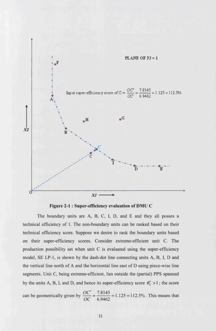
Figure 2-1 : Super-efficiency evaluation of DMU C
The boundary units are A, B, C, I, D, and E and they all posses a technical efficiency of 1. The non-boundary units can be ranked based on their technical efficiency score. Suppose we desire to rank the boundary units based on their super-efficiency scores. Consider extreme-efficient unit C. The production possibility set when unit C is evaluated using the super-efficiency model, SE LP-1, is shown by the dash-dot line connecting units A, B, I, D and the vertical line north of A and the horizontal line east of D using piece-wise line segments. Unit C, being extreme-efficient, lies outside the (partial) PPS spanned by the units A, B, I, and D, and hence its super-efficiency score 0*c >\ ', the score
O C' 7.8145
unit C can proportionately increase its input usage 1.125 times and still remain technically efficient. Carrying on in the above fashion, the super-efficiency score o f A is 1.3455, B is 1.0217, and D is 1.0667. The super-efficiency scores o f the boundary units that are not extreme-efficient, i.e., units I and E, are 1. Hence, based on the super-efficiency scores, unit A performs better than C, which performs better than D, and B performs the least best among the extreme- efficient units.
2.4.3 A b rief literature review on super-efficiency models
One can see from Thrall (1996b) as well as Banker and Chang (2006) that the idea o f super-efficiency was introduced much earlier in the article by Banker and Gifford (1989), an article that was th