SPICE
2
– A Spatial Parallel
Architecture for Accelerating the
SPICE Circuit Simulator
Thesis by
Nachiket Kapre
In Partial Fulfillment of the Requirements
for the Degree of
Doctor of Philosophy
California Institute of Technology
Pasadena, California
2010
c
2010
Nachiket Kapre
Abstract
Spatial processing of sparse, irregular floating-point computation using a single FPGA
enables up to an order of magnitude speedup (mean 2.8× speedup) over a
conven-tional microprocessor for the SPICE circuit simulator. We deliver this speedup
us-ing a hybrid parallel architecture that spatially implements the heterogeneous forms
of parallelism available in SPICE. We decompose SPICE into its three constituent
phases: Model-Evaluation, Sparse Matrix-Solve, and Iteration Control and parallelize
each phase independently. We exploit data-parallel device evaluations in the
Model-Evaluation phase, sparse dataflow parallelism in the Sparse Matrix-Solve phase and
compose the complete design in streaming fashion. We name our parallel
architec-ture SPICE2: Spatial Processors Interconnected for Concurrent Execution for ac-celerating theSPICE circuit simulator. We program the parallel architecture with a
high-level, domain-specific framework that identifies, exposes and exploits parallelism
available in the SPICE circuit simulator. Our design is optimized with an auto-tuner
that can scale the design to use larger FPGA capacities without expert intervention
and can even target other parallel architectures with the assistance of automated
code-generation. This FPGA architecture is able to outperform conventional
proces-sors due to a combination of factors including high utilization of statically-scheduled
resources, low-overhead dataflow scheduling of fine-grained tasks, and overlapped
processing of the control algorithms.
We demonstrate that we can independently accelerate Model-Evaluation by a
mean factor of 6.5×(1.4–23×) across a range of non-linear device models and
Matrix-Solve by 2.4×(0.6–13×) across various benchmark matrices while delivering a mean
Virtex-6 LX760 (40nm) with an Intel Core i7 965 (45nm). With our high-level
frame-work, we can also accelerate Single-Precision Model-Evaluation on NVIDIA GPUs,
ATI GPUs, IBM Cell, and Sun Niagara 2 architectures.
We expect approaches based on exploiting spatial parallelism to become
impor-tant as frequency scaling slows down and modern processing architectures turn to
parallelism (e.g. multi-core, GPUs) due to constraints of power consumption. Our
thesis shows how to express, exploit and optimize spatial parallelism for an important
Contents
Abstract iii
1 Introduction 1
1.1 Contributions . . . 2
1.2 SPICE . . . 7
1.3 FPGAs . . . 9
1.4 Implementing SPICE on an FPGA . . . 11
2 Background 15 2.1 The SPICE Simulator . . . 15
2.1.1 Model-Evaluation . . . 17
2.1.2 Matrix Solve . . . 19
2.1.3 Iteration Control . . . 20
2.2 SPICE Performance Analysis . . . 22
2.2.1 Total Runtime . . . 22
2.2.2 Runtime Scaling Trends . . . 23
2.2.3 CMOS Scaling Trends . . . 25
2.2.4 Parallel Potential . . . 26
2.3 Historical Review . . . 31
2.3.1 FPGA-based SPICE solvers . . . 35
2.3.2 Our FPGA Architecture . . . 36
3.1.1 Parallelism Potential . . . 41
3.1.2 Specialization Potential . . . 42
3.2 Related Work . . . 43
3.3 Verilog-AMS Compiler . . . 46
3.4 Fully-Spatial Implementation . . . 47
3.5 VLIW FPGA Architecture . . . 51
3.5.1 Operator Provisioning . . . 53
3.5.2 Static Scheduling . . . 55
3.5.3 Scheduling Techniques . . . 56
3.5.3.1 Conventional Loop Unrolling . . . 57
3.5.3.2 Software Pipelining with GraphStep Scheduling . . . 58
3.6 Methodology and Performance Analysis . . . 62
3.6.1 Toolflow . . . 62
3.6.2 FPGA Hardware . . . 63
3.6.3 Optimized Processor Baseline . . . 64
3.6.4 Overall Speedups . . . 65
3.6.5 Speedups for Different Verilog-AMS Device Models . . . 66
3.6.6 Effect of Device Complexity on Speedup . . . 68
3.6.7 Understanding the Effect of Scheduling Strategies . . . 71
3.6.8 Effect of PE Architecture on Performance . . . 72
3.6.9 Auto-Tuning System Parameters . . . 74
3.7 Parallel Architecture Backends . . . 76
3.7.1 Parallel Architecture Potential . . . 77
3.7.2 Code Generation . . . 80
3.7.3 Optimizations . . . 82
3.7.4 Auto Tuning . . . 82
3.8 Results: Single-Precision Parallel Architectures . . . 84
3.8.1 Performance Analysis . . . 85
3.8.2 Explaining Performance . . . 89
4 Sparse Matrix Solve 92
4.1 Structure of Sparse Matrix Solve . . . 92
4.1.1 Structure of the KLU Algorithm . . . 94
4.1.2 Parallelism Potential . . . 99
4.2 Dataflow FPGA Architecture . . . 103
4.3 Related Work . . . 108
4.3.1 Parallel Sparse Matrix Solve for SPICE . . . 108
4.3.2 Parallel FPGA-based Sparse Matrix Solvers . . . 109
4.3.3 General-Purpose Parallel Sparse Matrix Solvers . . . 110
4.4 Experimental Methodology . . . 111
4.4.1 FPGA Implementation . . . 114
4.5 Results . . . 115
4.5.1 Exploring Opportunity for Iterative Solvers . . . 115
4.5.2 Sequential Baseline: KLU withspice3f5 . . . 116
4.5.3 Parallel FPGA Speedups . . . 118
4.5.4 Limits to Parallel Performance . . . 121
4.5.5 Impact of Scaling . . . 124
4.6 Conclusions . . . 126
5 Iteration Control 127 5.1 Structure in Iteration Control Phase . . . 127
5.2 Performance Analysis . . . 129
5.3 Components of Iteration Control Phase . . . 132
5.4 Iteration Control Implementation Framework . . . 136
5.5 Hybrid FPGA Architecture . . . 138
5.6 Methodology and Results . . . 140
5.6.1 Integration with spice3f5 . . . 140
5.6.2 Mapping Flow . . . 141
5.6.3 Hybrid VLIW FPGA Implementation . . . 142
5.6.5 Comparing Application-Level Impact . . . 145
5.7 Conclusions . . . 147
6 System Organization 148 6.1 Modified SPICE Solver . . . 148
6.2 FPGA Mapping Flow . . . 149
6.3 FPGA System Organization and Partitioning . . . 152
6.4 Complete Speedups . . . 153
6.5 Comparing different Figures of Merit . . . 154
6.6 FPGA Capacity Scaling Analysis . . . 158
7 Conclusions 159 7.1 Contributions . . . 162
7.2 Lessons . . . 163
8 Future Work 165 8.1 Parallel SPICE Roadmap . . . 165
8.1.1 Precision of Model-Evaluation Phase . . . 165
8.1.2 Scalable Dataflow Scheduling for Matrix-Solve Phase . . . 166
8.1.3 Domain Decomposition for Matrix-Solve Phase . . . 166
8.1.4 Composition Languages for Integration . . . 166
8.1.5 Additional Parallelization Opportunities in SPICE . . . 167
8.2 Broad Goals . . . 168
8.2.1 System Partitioning . . . 168
8.2.2 Smart Auto-Tuners . . . 168
8.2.3 Fast Online Placement and Routing . . . 168
8.2.4 Fast Simulation . . . 170
8.2.5 Fast Design-Space Exploration . . . 170
8.2.6 Dynamic Reconfiguration and Adaptation . . . 171
Chapter 1
Introduction
This thesis shows how to expose, exploit and implement the parallelism available in
the SPICE simulator [1] to deliver up to an order of magnitude speedup (mean 2.8×
speedup) on a single FPGA chip. SPICE (Simulation Program with Integrated
Cir-cuit Emphasis) is an analog cirCir-cuit simulator that can take days or weeks of runtime
on real-world problems. It models the analog behavior of semiconductor circuits
us-ing a compute-intensive non-linear differential equation solver. SPICE is notoriously
difficult to parallelize due to its irregular, unpredictable compute structure, and a
sloppy sequential description. It has been observed that less than 7% of the
floating-point operations in SPICE are automatically vectorizable [2]. SPICE is part of the
SPEC92 [3] benchmark collection which is a set of challenge problems for
micropro-cessors. Over the past couple of decades, we have relied on innovations in computer
architecture (clock frequency scaling, out-of-order execution, complex branch
predic-tors) to speedup applications like SPICE. It was possible to improve performance of
existing application binaries by retaining the exact same ISA (Instruction Set
Archi-tecture) abstraction at the expense of area and power consumption. However, these
traditional computer organizations have now run up against a power wall [4] that
prevents further improvements using this approach. More recently, we have migrated
microprocessor designs towards “multi-core” organizations [5, 6] which are an
ad-mission that further improvements in performance must come from parallelism that
will be explicitly exposed to the hardware. Reconfigurable, spatial architectures like
SPICE Phase Description Parallelism Compute Organization Model Evaluation Verilog-AMS Data Parallel Statically-Scheduled VLIW
Matrix Solve Sparse Graph Sparse Dataflow Token Dataflow Iteration Control SCORE Streaming Sequential Controller
Table 1.1: Thesis Research Matrix
at lower clock frequencies and lower power. Unlike multi-core organizations which
can exploit a fixed amount of instruction-level parallelism, thread-level parallelism
and data-level parallelism, FPGAs can be configured and customized to exploit
par-allelism at multiple granularities as required by the application. FPGAs offer higher
compute density [7] by implementing computation using spatial parallelism which
distributes processing in space rather than time. In this thesis, we show how to
trans-late the high compute density available on a single-FPGA to accelerate SPICE by
2.8× (11× max.) using a high-level, domain-specific programming framework. The
key questions addressed in this thesis as follows:
1. Can SPICE be parallelized? What is the potential for accelerating SPICE?
2. How do we express the irregular parallel structure of SPICE?
3. How do we use FPGAs to exploit the parallelism available in SPICE?
4. Will FPGAs outperform conventional multi-core architectures for parallel SPICE?
We intend to use SPICE as a design-driver to address broader questions. How
do we capture, exploit and manage heterogeneous forms of parallelism in a single
application? How do we compose the parallelism in SPICE to build the integrated
solution? Is it sufficient to constrain this parallelism to a general-purpose architecture
(e.g. Intel multi-core)? Will the performance of this application scale easily with
larger processing capacities?
1.1
Contributions
We develop a novel framework to capture and reason about complex applications
expressing and unifying this parallelism effectively. We organize our parallelism on
reconfigurable architecture to spatially implement and customize the compute
orga-nization to each style of parallelism. We configure this hardware with a compilation
flow supported by auto-tuning to implement the parallelism in a scalable manner on available resources. We use SPICE as a design driver to experiment with these
ideas and quantitatively demonstrate the benefits of this design philosophy.
As shown in the matrix in Table 1.1, we first decompose SPICE into its three
constituent phases: (1) Model Evaluation, (2) Sparse Matrix-Solve and (3) Iteration
Control. We describe these phases in Chapter 2.
We identify opportunities for parallel operation in the different phases of SPICE
and provide design strategies for hardware implementation using suitable parallel
patterns. Parallel patterns are a paradigm of structured concurrent program-ming that help us express, capture and organize parallelism. Paradigms and patterns
were identified in the classic paper by Floyd [8]. They are invaluable tools and
tech-niques for describing computer programs in a methodical “top-down” manner. When
describing parallel computation, we need similar patterns for organizing our parallel
program. We can always expose available parallelism in the most general
Communi-cating Sequential Processes (CSP [9]) model of computation. However, this provides
no guidance for managing communication and synchronization between the parallel
processes. It also does not necessarily provide any insight into choosing the right
hardware implementation for the parallelism. In contrast, parallel patterns are reusable strategies for describing and composing parallelism that serve two key
pur-poses. First, these patterns let the programmer construct the parallel program from
well-known, primitive, building blocks that can compose with each other. Second,
the patterns also provide structure for constructing parallel hardware that best
im-plements the computation. This is more restricted than the general CSP model but
simplifies the task of writing the parallel program and developing parallel hardware
using well-developed solutions to avoid common pitfalls.
We analyze the structure of SPICE in the form of patterns and illustrate how
of SPICE can be effectively parallelized using the data-parallel pattern. We
imple-ment this data-parallelism in a software-pipelined fashion on the FPGA hardware.
We further exploit the static nature of this data-parallel computation to schedule the
computation on a custom, time-multiplexed, VLIW architecture. We extract the
ir-regular,sparse dataflowparallelism available in the Matrix-Solve phase of SPICE that
is different from the regular,data-parallelpattern that characterizes Model-Evaluation
phase. We use the KLU matrix-solver package to expose the static dataflow
paral-lelism available in this phase and develop a distributed, token-dataflow architecture
for exploiting that parallelism. This static dataflow capture allows us to distribute the
graph spatially across parallel compute units and process the graph in a fine-grained
fashion. Finally, we express the Iteration-Control phase of SPICE using a
stream-ing pattern in the high-level SCORE framework to enable overlapped evaluation and
efficiently implement the SPICE analysis state machines.
We now describe some key ideas that help us develop our parallel FPGA
imple-mentation:
• Domain-Specific Framework: The parallelism in SPICE is a heterogeneous
composition of multiple parallel domains. To properly capture and exploit
par-allelism in SPICE, we develop domain-specific flows which include high-level
lan-guages and compilers customized for each domain. We develop a Verilog-AMS
compiler to describe the non-linear differential equations for Model-Evaluation.
We use the SCORE [10] framework (TDF language and associated compiler
and runtime) to express the Iteration-Control phase of SPICE and compose the
complete design. This high-level problem capture makes the spatial, parallel
structure of the SPICE program evident. We can then use the compiler and
develop auto-tuners to exploit this spatial structure on FPGAs.
• Specialization: The SPICE simulator requires three inputs: (1) Circuit (2)
Device type and parameters (3) Convergence/Termination control options. We
exploit the static and early-bound nature of certain inputs to generate optimized
computation is dependent on device type and the device parameters. We can
pre-compile, optimize and schedule the static dataflow computation for the few
device types used by SPICE and simply select the appropriate type prior to
execution. We get an additional improvement in performance and reduction
in area by specializing the device evaluation to specific device parameters that
are common to specific semiconductor manufacturing processes. We quantify
the benefits of specialization in Table 3.4 in Chapter 3. The Sparse Matrix
Solve computation operates on a dataflow graph that can be extracted at the
start of the simulation. This early-bound structure of the computation allows
us to distribute and place operations on our parallel architecture once and then
reuse the placement throughout the simulation. We show a 1.35×improvement
in sequential performance of Matrix-Solve phase through specialization in
Ta-ble 4.5 from Chapter 4. Finally, the simulator convergence and terminal control
parameters are loaded into registers at the start of the simulation and are used
by the hardware to manage the SPICE iterations.
• Spatial Architectures: The different parallel patterns in SPICE can be efficiently implemented on customized spatial architectures on the FPGA. Hence,
we identify and design the spatial FPGA architecture to match the pattern of
parallelism in the SPICE phases. Our statically-scheduled VLIW architecture
delivers high utilization of floating-point resources (40–60%) and is supported
by an efficient time-multiplexed network that balances the compute and
com-municate operations. We use a Token-Dataflow architecture to spatially
dis-tribute processing of the sparse matrix factorization graph across the
paral-lel architecture. The sparse graph representation also eliminates the need for
address-calculation and sequential memory access dependencies that constrain
the sequential implementation. Finally, we develop a streaming controller that
enables overlapped processing of the Iteration Control computation with the
rest of SPICE.
fam-ily and require a complete redesign to scale to larger FPGA sizes. We are
inter-ested in developing scalable FPGA systems that can be automatically adapted
to use extra resources when they become available. For speedup calculations in
this thesis, our parallel design is engineered to fit into the resources available
on a single Virtex-6 LX760 FPGA. We develop an auto-tuner that enables easy
scalability of our design to larger FPGA capacities. Our auto-tuner explores
area-memory-time space to pick the implementation that fits available resources
while delivering the highest performance. The Model-Evaluation and
Iteration-Control phases of SPICE can be accelerated almost linearly with additional
logic and memory resources. With a sufficiently large FPGA we can spatially
implement the complete dataflow graph of the Model-Evaluation and
Iteration-Control computation as a physical circuit without using a time-shared VLIW
architecture. Furthermore, the auto-tuner can automatically choose the proper
configuration for this larger FPGA. This is relevant in light of the recently
an-nounced Xilinx Virtex-7 FPGA family [11] that has 2–3× the capacity of the
FPGA we use in this thesis. However, the Sparse Matrix-Solve phase will only
enjoy limited additional parallelism with extra resources. Additional research
into decomposed matrix solvers is necessary to properly scale performance on a
larger system.
The quantitative contributions of this thesis include:
1. Complete simulator: We accelerate the complete double-precision
implemen-tation of the SPICE simulator by 0.2-11.1×when comparing the Xilinx Virtex-6
LX760 (40nm technology node) with an Intel Core i7 965 processor (45nm
tech-nology node) with no compromise in simulation quality.
2. Model-Evaluation Phase: We implement the Model-Evaluation phase by
compiling a high-level Verilog-AMS description to a statically-scheduled custom
VLIW architecture. We demonstrate a speedup of 1.4–23.1× across a range of
non-linear device models when comparing Double-Precision implementations on
of 4.5–123.5×for a Virtex-5 LX330, 10.1–63.9× for an NVIDIA 9600GT GPU,
0.4–6×for an ATI FireGL 5700 GPU, 3.8–16.2×for an IBM Cell and 0.4–1.4×
for a Sun Niagara 2 architectures when comparing Single-Precision evaluation
to an Intel Xeon 5160 across these architectures at 55nm–65nm technology. We
also show speedups of 4.5–111.6× for a Virtex-6 LX760, 13.1–133.1× for an
NVIDIA GTX285 GPU and 2.8–1200×for an ATI Firestream 9270 GPU when
comparing Single-Precision evaluation to an Intel Core i7 965 on architectures
at 40–55nm technology.
3. Sparse Matrix-Solve Phase: We implement the sparse dataflow graph
rep-resentation of the Sparse Matrix-Solve computation using a dynamically-routed
Token Dataflow architecture. We show how to improve the performance of
irreg-ular, sparse matrix factorization by 0.6–13.4×when comparing a 25-PE parallel
implementation on a Xilinx Virtex-6 LX760 FPGA with a 1-core
implementa-tion on an Intel Core i7 965 for double-precision floating-point evaluaimplementa-tion.
4. Iteration-Control Phase: Finally, we compose the complete simulator along
with the Iteration-Control phase using a hybrid streaming architecture that
combines static scheduling with limited dynamic selection. We deliver 2.6×
(max 8.1×) reduction in runtime for the SPICE Iteration-Control algorithms
when comparing a Xilinx Virtex-6 LX760 with an Intel Core i7 965.
1.2
SPICE
We now present an overview of the SPICE simulator and identify opportunities for
parallel operation. At the heart of the SPICE simulator is a non-linear differential
equation solver. The solver is a compute-intensive iterative algorithm that requires an
evaluation of non-linear physical device equations and sparse matrix factorizations in
each iteration. When the number of devices in the circuit grows, the simulation time
will increase correspondingly. As manufacturing process technologies keep improving
larger circuits into a single chip. The ITRS roadmap for semiconductors [12, 13]
suggests that SPICE simulation runtimes for modeling non-digital effects [12] and
large power-ground networks [13] are a challenge. This will increase the size of the
circuits (N) we want to simulate. SPICE simulation time scales as O(N1.2) which outpaces the increase in computing capacity of conventional architecturesO(N0.96) as shown in Figure 1.1 (additional discussion in Section 2.2). Our parallel, single-FPGA
design scales more favorably with increasing circuit size as O(N0.7). We show the peak capacities of the processor and FPGA used in the comparison in Table 1.2. A
parallel SPICE solver will decrease verification time and reduce the time-to-market
for integrated circuits. However, as identified in [2] parallelizing SPICE is hard. Over
the past three decades, parallel SPICE efforts have either delivered limited speedups
or sacrificed simulation quality to improve performance. Furthermore, the techniques
and solutions are specific to a particular system and not easily portable to newer,
better architectures. The SPICE simulator is a complex mix of multiple compute
patterns that demands customized treatment for proper parallelization. After a careful performance analysis, it is clear that the Model Evaluation and Sparse
Matrix-Solve phases of SPICE are the key contributors to total SPICE runtime. We note that
the Model Evaluation phase of SPICE is in fact embarrassingly parallel by itself and
should be relatively easy to parallelize. We describe our parallel solution in Chapter 3.
In contrast, the Sparse Matrix-Solve phase is more challenging. This is one of the
key reasons why earlier studies were unable to parallelize the complete simulator.
The underlying compute structure of Sparse Matrix Solve is irregular, unpredictable
and consequently performs poorly on conventional architectures. Recent advances
in numerical algorithms provide an opportunity to reduce these limitations. We
use the KLU solver [14, 15] to generate an irregular, dataflow factorization graph
that exposes the available parallelism in the computation. We explain our approach
for parallelizing the challenge Sparse Matrix-Solve phase in Chapter 4. Finally, the
Iteration-Control phase of SPICE is responsible for co-ordinating the simulation steps.
While it is a tiny fraction of sequential runtime, it may become a non-trivial fraction
Iteration-101 102 103 104 105
80486PentiumPentium 2 Pentium 3Pentium 4 Xeon 5160Core i7
106 107 108 109
FLOPS
Transistors
N
0.96(a) CPU Double-Precision FLOPS
10-4 10-3 10-2 10-1 100
102 103 104 105
Runtime/Iteration (s)
Circuit Size
N
0.7N
1.2sequential CPU parallel FPGA
(b) SPICE Runtime
Figure 1.1: Scaling Trends for CPU FLOPS and spice3f5runtime
Family Chip Tech. Clock Peak GFLOPS Power
(nm) (GHz) (Double) (Watts)
Intel Core i7 965 45 3.2 25 130
Xilinx Virtex-6 LX760 40 0.2 26 20–30
Table 1.2: Peak Floating-Point Throughputs (Double-Precision)
Control phase of SPICE in Chapter 5. Finally, in Chapter 6 we discuss how to
integrate the complete SPICE solver on a single FPGA.
1.3
FPGAs
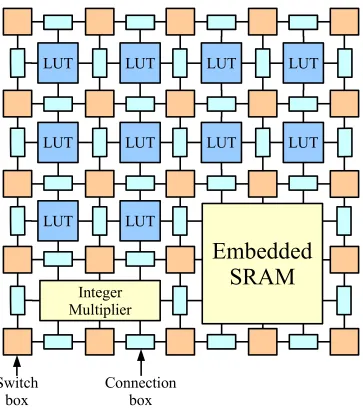
We briefly review the FPGA architecture and highlight some key characteristics of an
FPGA that make it well-suited to accelerate SPICE. A Field-Programmable Gate
Ar-ray is a massively-parallel architecture that implements computation using hundreds
of thousands of tiny programmable computing elements called LUTs (lookup tables)
connected to each other using a programmable communication fabric. Typically these
LUTs are clustered into SLICEs (2–4 LUTs per SLICE depending on FPGA
archi-tecture). Moore’s Law delivers progressively larger FPGA capacities with increasing
numbers of SLICEs per chip. Modern FPGAs also include hundreds of embedded
memories and integer multipliers distributed across the fabric for concurrent
LUT
LUT
LUT
LUT
LUT
LUT
LUT
LUT
LUT
LUT
Embedded
SRAM
Integer
Multiplier
Switch
[image:18.612.140.503.189.599.2]box
Connection
box
correspond to islands in a sea of interconnect). An FPGA allows us to configure
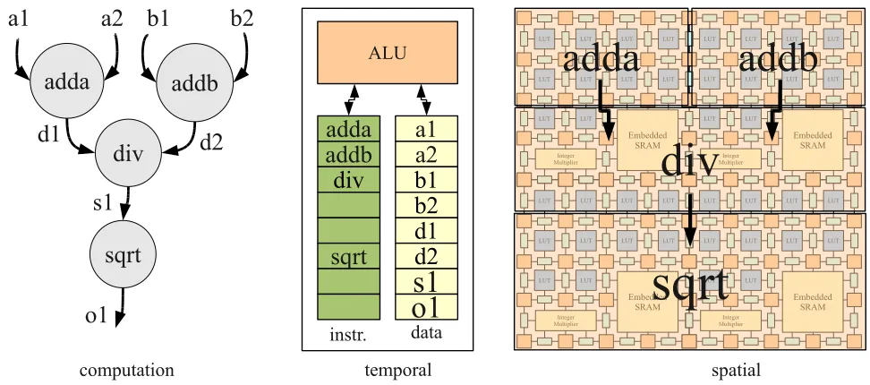
the computation in space rather than time and evaluate multiple operations
concur-rently in a fine-grained fashion. In Figure 1.3, we show a simple calculation and its
conceptual implementation on a CPU and an FPGA. For a CPU implementation, we
process the instructions stored in an instruction memory temporally on an ALU while
storing the intermediate results (i.e. variables) in a data memory. On an FPGA, we
can implement the operations as spatial circuits while implementing the dependencies
between the operations physically using pipelined wires instead of variables stored in
memory. Additionally a pipelined FPGA circuit implementation of certain operations
in the computation (e.g. divide, sqrt) require multiple cycles on the CPU while we
can configure a custom, pipelined circuit for those operations on the FPGA for higher
throughput.
While FPGAs have been traditionally successful at accelerating highly-parallel,
communication-rich algorithms and application kernels, they are a challenging
tar-get for mapping a complete application with diverse computational patterns such
as the SPICE circuit simulator. Furthermore, programming an FPGA with
exist-ing techniques for high performance requires months of effort and low-level tunexist-ing.
Additionally, these designs do not automatically scale for larger, newer FPGA
capac-ities that become available with technology scaling and require re-compilation and
re-optimization by an expert.
1.4
Implementing SPICE on an FPGA
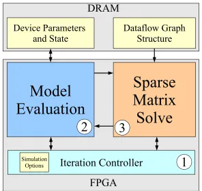
We now briefly describe our hardware architecture and mapping flow for implementing
SPICE on a single FPGA. We use a high-level framework to express, extract and
compose the parallelism in the different phases of SPICE. We develop a hybrid FPGA
architecture that combines custom architectures tailored to the parallelism in each
phase of SPICE. In Figure 1.4 we show a high-level block diagram of the composite
FPGA architecture with the three regions tailored for each phase of SPICE. We show
adda
addb
div
sqrt
adda
addb
div
sqrt
ALUa1
a2
b1
b2
d1
d2
s1
o1
a1
a2 b1
b2
[image:20.612.74.560.81.296.2]d1
d2
s1
o1
temporal spatial computation instr. data LUT LUT LUT LUT LUT LUT LUT LUT LUT LUT Embedded SRAM Integer Multiplier LUT LUT LUT LUT LUT LUT LUT LUT LUT LUT Embedded SRAM Integer Multiplier LUT LUT LUT LUT LUT LUT LUT LUT LUT LUT Embedded SRAM Integer Multiplier LUT LUT LUT LUT LUT LUT LUT LUT LUT LUT Embedded SRAM Integer Multiplieraddb
div
sqrt
adda
Figure 1.3: Implementing Computation
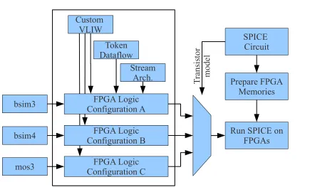
of the FPGA is the same for all SPICE circuits, we need to program the FPGA
memories in an instance-specific manner for each circuit we simulate. We show how
we assemble the FPGA hardware and provide additional details of our mapping flow
in Chapter 6.
A completely spatial implementation of the SPICE circuit simulator is too large
to fit on a single FPGA at 40nm technology today. On larger FPGAs, in the near
future, it will become possible to fit the fully-spatial Model Evaluation graphs entirely
on a single FPGA. For these graphs, the cost of a fully-spatial implementation gets
amortized across several device evaluations. However, for the Sparse Matrix-Solve
phase, the limited amount of parallelism and low reuse does not motivate a
fully-spatial design even if we have large FPGAs. Furthermore, configuring the FPGA
for every circuit using FPGA CAD tools (synthesize logic, place LUTs, and route
wires) can itself take hours or days of runtime defeating the purpose of a parallel
FPGA implementation for SPICE. We develop the custom FPGA architecture using
virtual organizations capable of accommodating the entire SPICE simulator operation
on a single FPGA. Furthermore, we simplify our circuit-specific compilation step by
Model
Evaluation
Device Parameters
and State
Sparse
Matrix
Solve
Dataflow Graph
Structure
Iteration Controller
2
3
1
SimulationOptions
DRAM
[image:21.612.176.472.79.358.2]FPGA
Figure 1.4: Block-Diagram of the SPICE FPGA Solver
SPICE Circuit
Prepare FPGA Memories FPGA Logic
Configuration A
Run SPICE on FPGAs Custom
VLIW
Token Dataflow
Stream Arch.
FPGA Logic Configuration B
FPGA Logic Configuration C
T
ra
ns
is
to
r
m
od
el
bsim3
bsim4
[image:22.612.125.560.247.510.2]mos3
Chapter 2
Background
In this chapter, we review the SPICE simulation algorithm and discuss the
inner-workings of the three constituent phases of SPICE. We review existing literature and
categorize previous attempts at parallelizing SPICE. We argue that these previous
approaches were unable to fully capitalize on the parallelism available within the
SPICE simulator due to limitations of hardware organizations and inefficiencies in
the software algorithms. In the following chapters, we will describe our FPGA-based
“spatial” approach that provides a communication-centric architecture for exploiting
the parallelism in SPICE.
2.1
The SPICE Simulator
SPICE simulates the dynamic analog behavior of a circuit described by its constituent
non-linear differential equations. It was developed at the EECS Department of the
University of California, Berkeley by Donald Pederson, Larry Nagel [1], Richard
New-ton, and many other contributors to provide a fast and robust circuit simulation
program capable of verifying integrated circuits. It was publicly announced
thirty-seven years ago in 1973 and many versions of the package have since been released.
spice2g6was part of the SPEC89 and SPEC92 benchmark sets of challenge problems for microprocessors. Many commercial versions of analog circuit simulators inspired
by SPICE now exist as part of a large IC design and verification industry. For this
Matrix A[i], Vector b [i]
Vector x [i] Vector x [i-1]
Model Evaluation Step (per device)
SPICE Iteration
Non-Linear Converged?
Increment timestep? Transient Iterations
Newton-Raphson Iterations
Matrix Solver A[i].x[i]=b[i] Matrix A[i], Vector b [i]
SPICE Deck: Circuit, Options
[image:24.612.164.487.80.363.2]Voltage, Current Waveforms
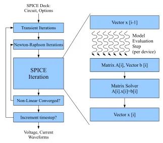
Figure 2.1: Flowchart of a SPICE Simulator
SPICE circuit equations model the linear (e.g. resistors, capacitors, inductors)
and non-linear (e.g. diodes, transistors) behavior of devices and the conservation
constraints (i.e. Kirchoff’s current laws—KCL) at the different nodes and branches
of the circuit. SPICE solves the non-linear circuit equations by alternately computing
small-signal linear operating-point approximations for the non-linear elements and
solving the resulting system of linear equations until it reaches a fixed point. The
linearized system of equations is represented as a solution of A~x = ~b, where A is the matrix of circuit conductances, ~b is the vector of known currents and voltage quantities and ~x is the vector of unknown voltages and branch currents.
Spice3f5 uses the Modified Nodal Analysis (MNA) technique [16] to assemble circuit equations into matrix A. The MNA approach is an improvement over conven-tional nodal analysis by allowing proper handling of voltage sources and controlled
current sources. It requires the application of Kirchoff’s Current Law at all the nodes
un-V1
D1
R1
+
_
GND
C1
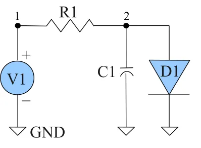
[image:25.612.230.429.84.230.2]1 2
Figure 2.2: SPICE Circuit Example
knowns for currents through branches to allow voltage sources and controlled current
sources to be represented.
The simulator calculates entries in Aand~bfrom the device model equations that describe device transconductance (e.g., Ohm’s law for resistors, transistor I-V
charac-teristics) in the Model-Evaluation phase. It then solves for~x using a sparse-direct linear matrix solver in the Matrix-Solve phase. We show the steps in the SPICE
algorithm in Figure 2.1. The inner loop iteration supports the operating-point
calcu-lation for the non-linear circuit elements, while the outer loop models the dynamics
of time-varying devices such as capacitors. The simulator loop management controls
are handled by the Iteration Control phase. We illustrate the operation of the
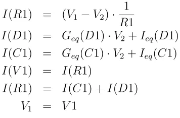
simulator using an example shown in Figure 2.2. We first write down the non-linear
differential equations that capture circuit behavior in Equation 2.1–Equation 2.6.
The non-linear (diode) and time-varying (capacitor) devices are represented using
linearized forms in Equation 2.2 and Equation 2.3 respectively. We then reassemble
these equations into A~x=~bform shown in Figure 2.4.
2.1.1
Model-Evaluation
In the Model-Evaluation phase, the simulator computes conductances and currents
through different elements of the circuit and updates corresponding entries in the
Fig-I(R1) = (V1−V2)· 1
R1 (2.1)
I(D1) = Geq(D1)·V2+Ieq(D1) (2.2)
I(C1) = Geq(C1)·V2+Ieq(C1) (2.3)
I(V1) = I(R1) (2.4)
I(R1) = I(C1) +I(D1) (2.5)
V1 = V1 (2.6)
Figure 2.3: Circuit Equations from Conservations Laws (KCL)
G1 −G1 1
−G1 G1 +Geq(C1) +Geq(D1) 0
1 0 0
×
V1
V2
I(V1)
=
0
Ieq(C1) +Ieq(D1)
V1
Figure 2.4: Matrix Representation of Circuit Equations in SPICE
ure 2.5 and fill-in the matrix appropriately in Figure 2.6. For the linear elements (e.g.
resistors) this needs to be done only once at the start of the simulation (shown in
blue in Figures 2.5 and 2.6). For non-linear elements, the simulator must search
for an operating-point using Newton-Raphson iterations which requires repeated
evaluation of the model equations multiple times per timestep (inner loop labeled
Newton-Raphson Iterations in Figure 2.1 and shown in red in Figure 2.5 and 2.6).
For time-varying components, the simulator must recalculate their contributions at
each timestep based on voltages at several previous timesteps. This also requires
repeated re-evaluations of the device-model (outer loop labeled Transient Iterations
in Figure 2.1 and shown in green in Figure 2.5 and 2.6).
I(R1) = (V1 −V2)·G1 (2.7)
I(C1) = (2·C1
δt )·V2−(
2·C1
δt ·V
old
2 +Iold(C1)) (2.8)
I(D1) = (Is
vj ·e
V2/vj)·V
[image:26.612.235.413.83.200.2]2+Is·(eV2/vj −1) (2.9)
G1 −G1 1
−G1 G1+(2·C1/δt) 0 +(Is/vj)·eV2/vj
1 0 0
· V1 V2
I(V1)
= 0
−((2·C1/δt)×Vold
2+Iold(C1))
+Is·(eV2/vj −1)
V1
[image:27.612.165.546.200.470.2]
Figure 2.6: Matrix contributions from the different devices
A·~x = ~b (2.10)
L·U·~x = ~b (2.11)
L·~y = ~b (2.12)
U·~x = ~y (2.13)
a11 a12 a13
a21 a22 a23
a31 a32 a33
· x1 x2 x3 = b1 b2 b3 (2.14)
1 0 0
l21 1 0
l31 l32 1
·
u11 u12 u13 0 u22 u23 0 0 u33
· x1 x2 x3 = b1 b2 b3 (2.15)
1 0 0
l21 1 0
l31 l32 1
· y1 y2 y3 = b1 b2 b3 (2.16)
u11 u12 u13 0 u22 u23 0 0 u33
· x1 x2 x3 = y1 y2 y3 (2.17)
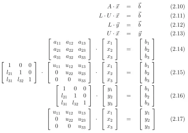
Figure 2.7: Matrix Solve Stages
2.1.2
Matrix Solve
The simulator spice3f5 uses the Modified Nodal Analysis (MNA) technique [16] to assemble circuit equations into matrix A. Since circuit elements (N) tend to be con-nected to only a few other elements, there are a constant number (O(1)) of entries per row of the matrix. Thus, the MNA circuit matrix with O(N2) entries is highly sparse with O(N) nonzero entries (≈99% of the matrix entries are 0). The matrix structure is mostly symmetric with the asymmetry being added by the presence of independent
sources (e.g. input voltage source) and inductors. The underlying non-zero
consequently remains unchanged throughout the duration of the simulation. In each
iteration of the loop shown in Figure 2.1, only the numerical values of the non-zeroes
are updated in the Model-Evaluation phase of SPICE with contributions from the
non-linear elements. To find the values of unknown node voltages and branch currents
~x, we must solve the system of linear equations A~x =~b as shown in Equation 2.14. The sparse, direct matrix solver used inspice3f5first reorders the matrixAto mini-mize fill-in using a technique called Markowitz reordering [17]. This tries to reduce the
number of additional non-zeroes (fill-in) generated during LU factorization. It then
factorizes the matrix by dynamically determining pivot positions for numerical
sta-bility (potentially adding new non-zeros) to generate the lower-triangular component
L and upper-triangular component U such that A=LU as shown in Equation 2.15. Finally, it calculates ~x using Front-SolveL~y =~b (see Equation 2.16) and Back-Solve U~x=~y operations (see Equation 2.17).
2.1.3
Iteration Control
The SPICE iteration controller is responsible for two kinds of iterative loops shown
in Figure 2.1: (1) inner loop: linearization iterations for non-linear devices and (2)
outer loop: adaptive time-stepping for time-varying devices. The Newton-Raphson algorithm is responsible for computing the linear operating-point for the non-linear
devices like diodes and transistors. Additionally, an adaptive time-stepping algorithm
based on truncation error calculation (Trapezoidal approximation, Gear
approxima-tion) is used for handling the time-varying devices like capacitors and inductors. The
controller also implements the loops in a data-dependent manner using customized
convergence conditions and local truncation error estimations.
Convergence Condition: The simulator declares convergence when two
con-secutive iterations generate solution vectors and non-linear approximations that are
within a prescribed tolerance respectively. We show the condition used by SPICE to
determine if an iteration has converged in Equation 2.18 and Equation 2.19. Here, V~i
or I~i represent the voltage or current unknowns in the i-th iteration of the
iteration (i) with the previous iteration (i−1). SPICE also performs a similar con-vergence check on the non-linear function described in the Model-Evaluation. The
closeness between the values in consecutive iterations is parametrized in terms of
user-specified tolerance values: reltol(relative tolerance), abstol(absolute tolerance), and vntol (voltage tolerance).
|V~i−V~i−1| ≤ reltol·max (|V~i|,|V~i−1|) +vntol (2.18)
|I~i−~Ii−1| ≤ reltol·max (|~Ii|,|I~i−1|) +abstol (2.19)
Typical values for these tolerances parameters are: reltol=1e−3 (accuracy of 1 part in 1000),abstol=1e−12 (accuracy of 1 picoampere) andvntol=1e−6 (accuracy of 1 µvolt). This means the simulator will declare convergence when the changes in voltage and current quantities get smaller than the convergence tolerances.
Local Truncation Error (LTE): Local Truncation Error is a local estimate
of accuracy of the Trapezoidal approximation used for integration. The
truncation-error-based time-stepping algorithm inspice3f5 computes the next stepsize δn+1 as a function of the LTE () of the current iteration and a Trapezoidal divided-difference approximation (DD3) of the charges (x) at a few previous iterations. The equation for stepsize is shown in Equation 2.20. For a target LTE, the Iteration Controller
can match the stepsize to the rate of change of circuit quantities. If the circuit
quantities are changing too rapidly, it can slow down the simulation by generating
finer timesteps. This allows the simulator to properly resolve the rapidly changing
circuit quantities. In contrast, if the circuit is quiescent (e.g. digital circuits between
clock edges), the simulator can take larger timesteps for a faster simulation. When
the change in the circuit quantities is small, a detailed simulation at fine timesteps
will be a waste of work. Instead, the simulator can advance the simulation with larger
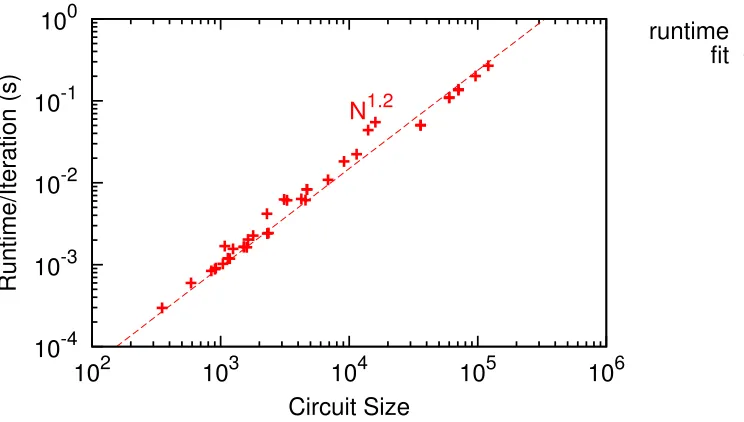
10-4 10-3 10-2 10-1 100
102 103 104 105 106
Runtime/Iteration (s)
Circuit Size
N1.2
[image:30.612.121.493.77.288.2]runtime fit
Figure 2.8: Sequential Runtime ofspice3f5for circuit benchmarks
δn+1 =
s
trtol· max (|DD3(x)|
12 , abstol)
(2.20)
tn+1 = tn+δn+1 (2.21)
2.2
SPICE Performance Analysis
In this section, we discuss important performance trends and identify performance
bottlenecks and characteristics that motivate our parallel approach. We usespice3f5 running on an Intel Core i7 965 for these experiments.
2.2.1
Total Runtime
We first measure total runtime of spice3f5 across a range of benchmark circuits on an Intel Core i7 965. We use a lightweight timing measurement scheme using
hardware-performance counters (PAPI [18]) that does not impact the actual runtime
of the program. We tabulate the size of the circuits used for this measurement along
with other circuit parameters in Table 4.2. We graph the runtimes as a function of
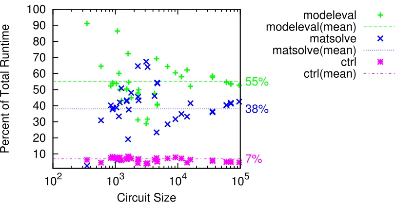
10 20 30 40 50 60 70 80 90 100
102 103 104 105
Percent of Total Runtime
Circuit Size
55%
38%
7%
[image:31.612.120.525.77.288.2]modeleval modeleval(mean) matsolve matsolve(mean) ctrl ctrl(mean)
Figure 2.9: Sequential Runtime Breakdown of spice3f5across the three phases
circuit sizeN. What contributes to this runtime? To understand this, we break down the contribution to total runtime from the different phases of SPICE in Figure 2.9.
We observe that, for most cases, total runtime is dominated by the Model-Evaluation
Phase. This is because the circuit is mostly composed of non-linear transistor
ele-ments. In some cases, the Sparse Matrix Solve phase can be a significant fraction of
total runtime. This is true for circuits with large parasitic components (e.g.
capaci-tors, resistors) where the non-linear devices are a small portion of total circuit size.
Finally, the control algorithm that sequences and manages SPICE iterations ends up
taking a small fraction of total runtime. This suggests that in our parallel solution
we must deliver high speedups for the intensive Model-Evaluation and Sparse Matrix
Solve phases of SPICE while ensuring that we do not ignore the control algorithms. If
we do not parallelize the Iteration Control phase, it may create a sequential bottleneck
due to Amdahl’s Law.
2.2.2
Runtime Scaling Trends
Why does SPICE runtime scale super-linearly when we increase circuit size? The
Model-Evaluation component of total runtime increases linearly with the number of
10-4 10-3 10-2 10-1 100
102 103 104 105
ModelEval Runtime/Iteration (ms)
Non-Linear Devices
N1.1
(a) Model-Evaluation Runtime
10-6 10-5 10-4 10-3 10-2 10-1
102 103 104 105
MatrixSolve Runtime/Iteration (ms)
Circuit Size
N1.2
(b) Matrix-Solve Runtime
Figure 2.10: Scaling Trends for the key phases of spice3f5
O(N) due to limited cache capacity of the processor; also see Figure 2.13(a)) as shown in Figure 2.10(a). The Matrix-Solve component of runtime empirically grows
as O(N1.2) as shown in Figure 2.10(b) (also see Figure 2.13(b) for floating-point operation trends). Overall, we observe from Figure 2.8 that runtime grows asO(N1.2) where N is the size of the circuit.
What other factors impact overall runtime? In Figure 2.11(a), we observe that
floating-point instructions constitute only≈20%–40% of total instruction count (smaller
fraction for larger circuits). The remaining instructions are integer and memory
ac-cess operations that support the floating-point work. These instructions are purely
overhead and can be implemented far more efficiently using spatial FPGA
hard-ware. They also consume instruction cache capacity and issue bandwidth, limiting
the achievable floating-point peak. Furthermore, we observe that increasing circuit
sizes results in higher L2 cache misses. We see L2 cache miss rates as high as 30%–
70% L2 for our benchmarks in Figure 2.11(b). As we increase circuit size, the sparse
matrix and circuit vectors spill out of the fixed cache capacity leading to a higher
cache miss rate. For the benchmarks we use, the sparse matrix storage exceeds the
256KB per-core L2 cache capacity of an Intel Core i7 965 for all except a few small
benchmarks. We also show the overflow factor (Memory required/Cache size) for our
10 20 30 40 50 60 70 80 90 100
102 103 104 105
Floating-Point Percent
Circuit Size
(a) Floating-Point Instruction Fraction
20 30 40 50 60 70 80
102 103 104 105
0.01 0.1 1 10 100
Cache Miss Percent
Cache Overflow Factor
Circuit Size
(b) L2 Cache Miss Rate
Figure 2.11: Instruction and Memory Scaling Trends for spice3f5
opportunity to properly distribute data across multiple, onchip, embedded memories
and manage communication operations (i.e. moving data between memories) to
de-liver good performance. Our FPGA architecture exploits spatial parallelism, even
in the non-floating-point portion of the computation, to deliver high speedup.
2.2.3
CMOS Scaling Trends
As we continue to reap the benefits of Moore’s Law [19], we need to simulate
increas-ingly larger circuits using SPICE. As we saw in the previous Section 2.2.2, sequential
SPICE runtimes scales asO(N1.2) where N=size of the circuit. This means sequential SPICE runtimes will get increasingly slower as we scale to denser circuits.
Further-more, as we shrink device feature sizes to finer geometries, we must model
increas-ingly detailed physical effects in the analog SPICE simulations. This will increase the
amount of time spent performing Model-Evaluation [20] as shown in Figure 2.12(a).
For example, the mos1MOSFET model implements the Shichman-Hodges equations which are adequate for discrete transistor designs. The semi-empirical mos3 model was originally developed for integrated CMOS short-channel transistors at 1–2µm or larger. The new bsim3v3 and bsim4 models are more accurate and commonly used for today’s technology. It may become necessary to use different models for RF
10 100 1000 10000
10 100 1000
Sequential CPU Time/Device (ns)
Device Parameters (Complexity) jfet bjt
bsim3 bsim4 psp mextram
mos1
mos3 vbic
hbt
(a) Impact of Non-Linear Device Complexity
101 102 103 104 105 106
ram2k ram8k ram64k
SPICE Runtime/Iteration (ns)
Circuits without parasitics
with parasitics
(b) Impact of Parasitics
Figure 2.12: Impact of CMOS Scaling on SPICE
At smaller device sizes, our circuits will suffer the impact of tighter coupling
and interference between the circuit elements. This will add additional modeling
requirement of parasitic elements (e.g. capacitors, resistors) which increase the size
of the matrix. This will, in turn, increase the time spent in the Sparse Matrix-Solve
phase. The increase in SPICE runtime per iteration due to inclusion of parasitic
effects is shown in Figure 2.12(b).
2.2.4
Parallel Potential
We now try to identify the extent of parallelism available in the two
computationally-intensive phases of SPICE. In Figure 2.13(a), we plot the total number of
floating-point operations as well as the latency of the Model-Evaluation computation assuming
ideal parallel hardware as a function of the number of non-linear elements in the
circuit. The amount of work grows linearly (O(N)) with the number of non-linear devices. However, the latency of the evaluation remains unchanged at the latency
of a single device evaluation. Each non-linear device can be independently evaluated
with local terminal voltages as inputs and local currents and conductances as outputs.
Thus, the amount of parallelism is proportional to the number of non-linear devices
in the circuit. This phase is embarrassingly parallel, and we show how to exploit this
104
105
106
107
108
101 102 103 104 105
101
102
103
104
105
Operations Latency
Non-Linear Circuit Elements
N1
N0
work fit(work) latency fit(latency)
(a) Total Work and Critical Latency Trends for the Model-Evaluation Phase
103 104 105 106 107
101 102 103 104 105
102 103 104 105 106
Operations Latency
Circuit Size
N1.4
N0.7
work fit(work) latency fit(latency)
[image:35.612.134.391.390.602.2](b) Total Work and Critical Latency Trends for the Matrix-Solve Phase
In Figure 2.13(b), we plot the total number of floating-point operations in the
Sparse Matrix-Solve phase of SPICE as well as the critical path latency as a function
of circuit size. Here, we observe that the amount of work in the sparse factorization
increases as O(N1.4) (compared to O(N3) for dense factorization). This growth rate is an empirical observation that is valid for circuit matrices in our benchmark set
(see [21]). This explains theO(N1.2) growth in total runtime we previously observed in Figure 2.8. The critical path latency of the factorization only grows as O(N0.7). This suggests that a well-designed parallel architecture can extract parallelism from
this phase since the critical path is not growing as fast asN. An architecture with low-latency communication and lightweight fine-grained spatial processing of operations
Y ear Ref. Name Key Idea P arallel Hardw are Sequen tial Baseline PEs Sp eedup SPICE phase Expression
Accuracy Tradeoff
1979 [22] -Static Dataflo w -100 72.8 Matrix Solv e Dataflo w graph None 1985 [23] -V ector task graph S810 vector S810 scalar 4 8.9 Matrix Solv e V ectorized graph None 1986 [24] Ca yenne Run time Sc heduling V AX 8800
scalar (spice2
Y ear Ref. Name Key Idea P arallel Hardw are Sequen tial Baseline PEs Sp eedup SPICE phase Expression
Accuracy Tradeoff
[image:38.612.114.522.45.725.2]Recen t Approac hes 2000 [35] Xyce Iterativ e Ma-trix Solv e SGI Origin 2000 1 PE 40 24 All Message-P assing (MPI) None 2002 [36] SMP- SPICE Multi- threading Hitac hi 900 0 N4000 1 thread 8 4.6 All C with PThreads None 2006 [37] SILCA Appro x. -1 thread spice3 1 7.4 All Sequen tial co de PWL, etc 2007 [38] Op enMP-SPICE Data-P arallel UltraSP AR C 3 1 thread spice3 4 1.3 Mo del Ev al. spice3f5 with Op enMP None 2008 [39] W av epip e Sp eculativ e P arallelism 4 dual-core SMP 1 thread 8 2.4 Iter. Ctrl Explicit PThreads None 2009 [40] A CCIT-NSR Data-parallel A TI Fire-Stream 9170 4-core AMD Phenom 320 50 Mo del Ev al. Data-parallel Bro ok [41] None 2009 [42] Nascen tric Data-parallel NVIDIA 8800 GTS 1-core In tel Core2 128 3 Mo del Ev al. Data-P arallel CUD A [43, 44] Single- Precision 2009 [45] DD Domain- Decomp osition FW Grid [46] 1 thread spice3f5 32 119 Matrix Solv e C with PETSc [47] pac kage None FPGA-based Approac hes 1995 [48] TINA based on A WSIM-3 23 Xilin x X C4005 chips -All Microasm As-sem bly T able-lo okup 1997 [49] -partial-ev al Altera Flex10K SP AR C sta-tion 3 27.7 Mo del Ev al. PECompiler C subset
Fixed- poin
t 2003 [50] SPO analytical transform Xilinx Spar-tan 3 -All Sim ulink graphs
fixed- poin
2.3
Historical Review
We now review the various studies and research projects that have attempted to
par-allelize SPICE in the past three decades or so. These studies attempt to accelerate the
computation using a combination of parallel hardware architectures and/or numerical
software algorithms that are more amenable to parallel evaluation. We tabulate and
classify these approaches in Table 2.1 and Table 2.2. We can refine the classification
of parallel SPICE approaches by considering underlying trends and characteristics of
the different systems as follows:
1. Compute Organization: We see parallel SPICE solvers using a range of
different compute organizations including conventional processing,
multi-core, VLIW, SIMD and Vector.
2. Precision: Under certain conditions, SPICE simulations can efficiently model
circuits at lower precisions.
3. Compiled Code: In many cases, it is possible to generate efficient
instance-specific simulations by specializing the simulator for a particular circuit.
4. Scheduling: Parallel computation exposed in SPICE must be distributed
across parallel hardware elements for faster operation. Many designs develop
novel, custom scheduling solutions that are applicable under certain structural
considerations of the circuit or matrix.
5. Numerical Algorithms: Different classes of circuits perform better with a
suitable choice of a matrix factorization algorithm. Our FPGA design may
benefit from new ideas for factoring the circuit matrix.
6. SPICE Algorithms: Conventional SPICE simulations often perform needless
computation across multiple iterations that is not strictly necessary for an
ac-ceptable result. In many cases, it is possible to rapidly advance simulation time
paral-lel FPGA system can enjoy the benefits of exposing paralparal-lelism in the iteration
management algorithms.
We now roughly organize the evolution of parallel SPICE systems into five ages
and identify the appropriate category for the systems considered:
Age of Starvation (1980-1990): In the early days of VLSI scaling, the amount of computing resources available was limited. This motivated designs of custom
ac-celerator systems for SPICE that were assembled from discrete components (e.g. [25,
51, 26]). Numerical algorithms for SPICE were still being developed and not directly
suitable for parallel evaluation. The systems scavenged parallelism in SPICE using
compiled-code approaches and customized hardware. In a compiled-code approach,
the framework produces code for an instance of the circuit and compiles this
gen-erated code for the target architecture. This exposes instance-specific parallelism in
SPICE to the compiler in two primary ways: (1) it enables static optimization of
recurring, redundant work in the Model Evaluation phase and (2) it disambiguates
memory references for the sparse matrix access. The resulting compiled-code
pro-gram is capable of only simulating the particular circuit instance. One of the earliest
papers [22] on parallel SPICE sketches a design for the sparse matrix-solve phase by
extracting the static triangulation graph for the matrix factorization but ignores
com-munication costs. Other studies have also considered extracting the static dataflow
graph for matrix factorization using the MVA (Maximal Vectorization Algorithm)
approach [23] (Compiled Code). The resulting graph is vectorized onto a Hitachi
S810 supercomputer to get a 8.9× speedup with 4 vector units and a modest increase
in storage of intermediate results. Vectorization and simpler address calculation are
key reasons for this high speedup. Cayenne [24] maps the SPICE computation to
a 2-processor VAX system (Compute Organization) running a multiprocessing
operating-system VMS but achieves a limited speedup of 1.7×. A custom design for
a SPICE accelerator with 2 PEs [25] running a Compiled Code SPICE simulation
shows a speedup of 2×over a VAX 8650 operating at ≈2× the frequency. It
empha-sizes parallelizing addressing and memory lookup operations within the Processing
Com-piled Codesimulator outlined in [26] delivers a speedup of 7.3×using 6 processors.
This approach exploits multiple levels of granularity in the sparse matrix solve and
optimizes locking operations in model-evaluation for greater parallelism. However,
performance is constrained by the high operand storage costs of applying a
compiled-code methodology to the complete simulator on processing architecture with limited
memory resources.
Age of Growth (1991-1995): As silicon capacity increased, we saw improved parallel SPICE solvers based on vector or distributed-memory architectures (e.g. [27,
31, 33]). These systems were more general-purpose than the custom accelerators.
However, they required careful parallel programming, performance tuning and novel
scheduling algorithms to manage parallelism. Awsim-3 [51, 28] again uses a
Com-piled Codeapproach and a special-purpose system (Compute Organization) with
table-lookup (Precision) Model-Evaluation to provide a speedup of 560×over a Sun
3/60. The Sun 3/60 implements floating-point operations in software which takes
tens of cycles/operation. This means that a bulk of the speedup comes from
hard-ware floating-point units in Awsim-3. Another scheme presented in [27] schedules
the complete SPICE computation as a homogeneous graph of tasks (Scheduling).
It delivers a speedup of 4.5× on 8 processors. Parallel waveform-relaxation (SPICE
Algorithms) is considered in [29] and [30] and demonstrates good speedups using the different simulation algorithm. A novel row-scheduling algorithm (Scheduling)
for processing the sparse matrix solve operations is presented in [31] to obtain modest
speedups of 3.7× on 4 processors. A preconditioned Jacobi technique (Numerical
Algorithms) for matrix solve is discussed in [32] but achieves speedups of 16.5×using 64 processors. This is due to the cost of calculating and applying the preconditioner.
In [33], the task scheduling algorithm extracts fine-grained tasks (Scheduling) from
the complete SPICE computation to achieve an unimpressive speedup of 4.3×
us-ing 8 processors. Transputers have been used for acceleratus-ing block-decomposition
factorization (Numerical Algorithms) for the sparse matrix solve phase of SPICE
Age of the “Killer Micros” (1996-2005): Moore’s law of VLSI scaling had
fa-cilitated the ascendance of general-purpose ISA (Instruction Set Architecture)
unipro-cessors. These “killer micros” [52, 53] rode the scaling curve across technology
gener-ations and delivered higher compute performance while retaining the ISA
program-ming abstraction. Processors now included integrated high-performance
floating-point units which enabled them to deliver SPICE performance that was competitive
with custom accelerators. As a result, this age is characterized by a lack of many
significant breakthroughs in parallel SPICE hardware designs. A notable exception
is the mapping of parallel SPICE to an SGI Origin 2000 supercomputer with 40
nodes (MIPS R10K processors) in [35]. The supercomputer (Compute
Organiza-tion) was able to speedup SPICE for certain specialized benchmarks by 24× using a message-passing description of SPICE.
Age of Plenty (2006-2010): In this age, the uniprocessor era was starting to run out of steam. The cost of retaining the ISA abstraction while delivering frequency
improvements was increasing power consumption to unsustainable levels. This meant
that it was no longer possible to simply scale frequency or superscalar
Instruction-Level Parallelism to deliver higher performance. The microprocessor vendors turned
to putting multiple parallel “cores” on a chip and transferred the responsibility of
performance improvement to the programmer. Thus, it became important to
explic-itly expose parallelism to get high performance. A few studies accelerated SPICE
by a modest amount on such systems using multi-threading (e.g. [36, 38]). This
age also saw the rise of the Graphics Processing Units (GPUs) for general-purpose
computing (GP-GPUs) which densely packed hundreds of single-precision
floating-points on a single chip. A few studies (e.g. [40, 42]) have shown great speedups when
accelerating the Model-Evaluation phase of SPICE using GPUs (Compute
Organi-zation). In [36], a multi-threaded version of SPICE is developed using coarse-grained
PThreads. It achieves a speedup of 5×using 8 SMP (Symmetric Multi-Processors) on
a small benchmark set. SILCA [37] delivers good speedup for circuits with parasitic
couplings (resistors and capacitors) using a combination of low-rank matrix updates,
Numer-ical Algorithms). It is possible to achieve limited speedups of 1.3× for SPICE
shown in [38] using OpenMP pragma annotations to the Model-Evaluation portion of
existing SPICE source-code. GPUs can be used to speedup the data-parallel
Model-Evaluation phase of SPICE by 50×([40]) or 32×([42]) but can accelerate the
com-plete SPICE simulator in tandem with the CPU by 3× for the GPU-CPU system.
A speedup of 2.4× can be achieved using speculative execution of multiple timesteps
as demonstrated in [39] (SPICE Algorithms). This approach is orthogonal to the
technique discussed in this thesis and can be used to extend our speedups further with
additional hardware. In [45], the authors show a speedup of 119×using 32 processors
with a domain-decomposition approach (Numerical Algorithms) for accelerating
Sparse Matrix-Solve phase. This technique breaks up a large circuit matrix into
smaller overlapping submatrices and factorizes them independently. This idea, too,
is orthogonal to our approach where we can use our FPGA-based solver to accelerate
the individual submatrices.
Age of Efficiency (2010-beyond)As Moore’s Law starts to hit physical limits of energy and reliability, we must seek novel architectures for organizing computation.
The ISA abstraction is power-hungry and wasteful of silicon resources. Multi-core
architectures will eventually run into power-density limits at small feature sizes [54].
The simple SIMD model in GP-GPUs is unsuitable for sparse, irregular computation
(e.g. Sparse Matrix-Solve). Instead, we must consider energy-efficient, high-density
reconfigurable architectures (e.g.FPGAs) for implementing computation. We need to
create customized architectures that match the parallel patterns in SPICE to get high
performance. Communication bandwidth and latency become first-class concerns in
the compilation flow. This thesis shows how to express, exploit and implement the
parallelism available in SPICE using custom FPGA architectures.
2.3.1
FPGA-based SPICE solvers
FPGAs have been used extensively in custom-computing machines for accelerating a
wide variety of compute-intensive applications. However, they have enjoyed limited
methodology for attacking a problem of this magnitude. In this context, FPGAs
were first used in a SPICE accelerator asglue logic[31] to implement the VME
inter-face (Versa Module Europa, IEEE 1014-1987 bus standard) and store communication
schedules to support a 4-chip Intel i860 system with a Compiled Code approach.
The schedules are implemented using an FPGA-based sequencer. The design in [48]
used FPGAs to support the VLIW datapath for accelerating SPICE. Due to limited
FPGA capacity, the FPGA was connected to discrete Weitek floating-point units
and SRAM chips (Compute Orgnization). A Compiled Code, partial
evalua-tion approach for timing simulaevalua-tion (lower precision than SPICE) using FPGAs was
demonstrated in [49] where the processing architecture was customized for a
par-ticular SPICE circuit. The compiler generates optimized fixed-point function units
(Precision) and schedules memory access for the simulation. Fixed-point
compu-tation may be unsuitable for certain simulation scenarios with high-dynamic range
of physical quantities (e.g. leakage simulations with picoampere resolutions).
Ad-ditionally, this approach demands that the physical FPGA be configured for every
circuit being simulated. FPGA mapping algorithms are time-consuming and may
themselves take hours to days of runtime. Another recent study [50] explores the
use of an FPGA-based, SPICE-like simulator for speeding up transient simulations of
SPICE circuits expressed as digital signal processing objects (SPICE Algorithms).
This approach converts an analytical analog representation of circuit equations into a
graph of variable-rate, discretized, streaming operators. The accuracy of the solution
depends on the discretization algorithm (Precision) and may require extremely fine
timesteps for correct convergence. Moreover, the current implementation operates on
8-bit/16-bit data-types which are insufficient for detailed leakage simulations.
2.3.2
Our FPGA Architecture
We now highlight some key features of our architecture that are inspired by the
previ-ous studies or superior to the older approaches as appropriate. Our FPGA-based
table-lookups) or reducing the amount of computation (e.g.low-rank updates) is orthogonal
to our approach under identical convergence and truncation requirements. We use a
Compiled Codeapproach similar to several previous studies for our design. We
cap-ture parallelism available in the SPICE simulator using a high-level, domain-specific
framework that supports a compiled-code methodology for optimizing the simulation.
We then implement this parallelism on available FPGA resources by choosing how to
spread this parallelism spatially across the FPGA fabric (Compute Organization)
while distributing memory accesses over embedded, distributed memories. We are
also able to exploit additional parallelism by building custom architectures that are
tailored to unique forms of parallelism specific to each SPICE phase. Previous studies
did not to change their compute organization to adapt to the parallelism for each of
the three phases of SPICE. Our approach considers communication as a first-class
concern and designs high-bandwidth, low-latency networks that use either a
time-multiplexed approach for Model-Evaluation or a dynamically-routed packet-switched
design for the Sparse Matrix-Solve. Previous studies either used expensive crossbars
or slow packet-switched networks to support communication traffic. We distribute
the computation for locality and tune network bandwidth when required to balance
Chapter 3
Model-Evaluation
In Chapter 2 (Section 2.1), we introduced Model Evaluation as an easily parallelizable
phase of the SPICE circuit simulator. It is characterized by abundant data parallelism
where each device can be evaluated concurrently in a data-independent manner. In
this chapter, we first identify additional computational characteristics of the
Model-Evaluation phase that are important for an efficient parallel mapping. We show how
to compile the non-linear differential equations describing SPICE device models
us-ing a high-level, domain-specific framework based on Verilog-AMS. We then sketch
a hypothetical fully spatial design that distributes the complete Model-Evaluation
computation in space as a configured circuit to achieve the highest throughput. We
develop spatial organizations that can be realized on a single FPGA using
statically-scheduled time-multiplexing of FPGA resources. This allows us to use less area than
the fully spatial