Extremal Combinatorics
Matthew Jenssen
A thesis submitted for the degree of Doctor of Philosophy
Department of Mathematics London School of Economics
and Political Science
I certify that the thesis I have presented for examination for the PhD degree of the London School of Economics and Political Science is my own work other than where I have clearly indicated that it is the work of others (in which case the extent of any work carried out jointly by me and any other person is clearly identified in it).
The copyright of this thesis rests with the author. Quotation from it is permitted, provided that full acknowledgement is made. This thesis may not be reproduced without the prior written consent of the author.
In this thesis we explore instances in which tools from continuous optimi-sation can be used to solve problems in extremal graph and hypergraph theory.
We begin by introducing a generalised notion of hypergraph Lagrangian and use tools from the theory of nonlinear optimisation to explore some of its properties. As an application we find the Tur´an density of a small family of hypergraphs.
We determine the exact k-colour Ramsey number of an odd cycle on n
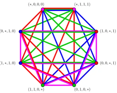
vertices when n is large. This resolves a conjecture of Bondy and Erd˝os for large n. The first step of our proof is to use the regularity method to relate this problem in Ramsey theory to one in nonlinear optimisation. We establish a correspondence between extremal constructions in the Ramsey setting and optimal points in the continuous setting. We thereby uncover a correspondence between extremal constructions and perfect matchings in thek-dimensional hypercube. This allows us to prove a stability type result around these extremal constructions.
We consider two models from statistical physics, the hard-core model and the monomer-dimer model. Using tools from linear programming we give tight upper bounds on the logarithmic derivative of the independence and matching polynomials of a d-regular graph. For independent sets, this is a strengthening of a sequence of results of Kahn, Galvin and Tetali, and Zhao that a disjoint union ofKd,d’s maximises the independence polynomial
and total number of independent sets among all d-regular graphs on the same number of vertices. For matchings, the result implies that disjoint unions ofKd,d’s also maximise the matching polynomial and total number of matchings. Moreover we prove the Asymptotic Upper Matching Conjecture of Friedland, Krop, Lundow, and Markstr¨om.
I would like to thank my supervisors Julia B¨ottcher and Jozef Skokan for providing me with support, encouragement and fascinating mathematical problems throughout my time as a PhD student.
I would like to thank the staff and faculty of the LSE Mathematics de-partment for providing a welcoming and wonderful work environment. In particular I would like to thank Rebecca Lumb and Kate Barker for their endless help and motivational chocolates.
I would like to thank my PhD colleagues, Ewan Davies and Barnaby Roberts, for the constant source of mathematical discussion and coffee time puzzles. I would also like to thank Will Perkins for inspiring me with his energetic and creative approach to mathematics and for being a wonderful collaborator.
I am grateful for the funding provided by my LSE PhD Studentship.
I would like to thank my parents, whose unwavering support and faith in me made it possible for me to pursue my passions. Without them, this would not have been possible.
1 Introduction 6
1.1 Notation and Terminology . . . 8
1.2 Extremal Hypergraph Theory . . . 10
1.2.1 Hypergraph Lagrangians . . . 12
1.3 Ramsey Theory . . . 14
1.4 Statistical Physics Models on Graphs . . . 18
1.5 Tools from Continuous Optimisation . . . 23
1.5.1 Linear Programming . . . 23
1.5.2 Karush-Kuhn-Tucker Conditions . . . 25
2 A Generalised Notion of Hypergraph Lagrangian 27 2.1 Introduction . . . 28
2.2 The Generalised Lagrangian . . . 30
2.3 1-avoiding 3-graphs and a proof of Theorem 2.1. . . 33
2.4 The GeneralisedK4 . . . 37
2.5 (r−2)-avoidingr-graphs for larger. . . 38
3 Ramsey Numbers Via Nonlinear Optimisation 42 3.1 Introduction . . . 43
3.2 A Graph Decomposition, Extremal Colourings and Stability . 48 3.2.1 A Graph Decomposition . . . 48
3.2.2 Extremal Colourings and the Hypercube . . . 48
3.2.3 Stability . . . 50
3.2.4 Proof of Theorem 3.4: An Overview . . . 51
3.3 Deriving the Analytic Constraints . . . 53
3.4 Compressions and a Spherical Constraint . . . 59
3.6 Towards an Exact Result: Analytic and Combinatorial Stability 74
3.7 The Regularity Method . . . 78
3.8 Proof of Main Theorem . . . 80
4 Independent Sets and the Hard-Core Model 95 4.1 Introduction . . . 96
4.1.1 Independent Sets in Regular Graphs . . . 96
4.1.2 Independent Sets in Triangle-Free Graphs . . . 97
4.2 Occupancy Fraction in Triangle-Free Graphs . . . 100
4.3 Counting Independent Sets in Triangle-Free Graphs . . . 105
4.4 Proof of Theorem 4.1 . . . 106
4.4.1 The Linear Program . . . 109
4.5 On the Ratio of the Maximum and Average Independent Set Size . . . 111
5 Matchings and the Monomer-Dimer Model 113 5.1 Introduction . . . 114
5.2 Proof of Theorem 5.1 . . . 115
5.2.1 The Linear Program for Matchings . . . 118
5.3 Matchings of a Given Size . . . 126
Bibliography 131 Appendices 139 A Completing the Proof of Theorem 2.1 . . . 139
1
Extremal graph theory concerns itself with problems of the following type:
Question A: Given a real-valued graph parameterP and a class of graphsC, how large (or small) canP be for an element ofC?
One of the earliest results in extremal graph theory is Mantel’s theorem [67] from 1907, which considers the case where C is the class of all triangle-free graphs onnvertices andP is the number of edges of a graph. Indeed, Man-tel’s theorem asserts that any triangle-free graph onnvertices must have at most bn2/4c edges. If we can answer Question A, we may want to go fur-ther and determine precisely which elements ofCoptimiseP. In the example of Mantel’s theorem, one can show that the complete, balanced, bipartite graph on n vertices, is the unique triangle-free graph on n vertices with bn2/4c edges. We call the graphs in C which optimise P extremal graphs. Once we have determined these extremal graphs, a curious phenomenon of-ten occurs. Ofof-ten one can show that elements ofCwhich almost optimiseP, must beclose (in some combinatorial sense) to one of our extremal elements ofC. We call this phenomenoncombinatorial stability.
Extremal graph theory can be viewed as ‘discrete optimisation’ where a natural continuous analogue might be a question of the following form:
Question B: Given a functionf :Rn→Rand a subsetS ⊆Rn, how large (or small) canf(x) be for an elementx∈S?
We will call a question of this type a question in continuous optimisation. If we can answer Question B, again we may want to know precisely which elements ofS optimise f. We call elements of S which optimise f optimal points. Similarly to the discrete case, one can often show that elements ofS
that almost optimisef must be close (in Euclidean distance say) to a genuine optimal point ofS. We refer to this phenomenon asanalytic stability.
century by Newton and Leibniz, many powerful new techniques to attack problems in continuous optimisation emerged. Euler and Lagrange were early pioneers in the general theory of continuous optimisation and by now there are many sophisticated tools to deal with questions of type B.
In this thesis, we explore instances in which problems in extremal graph (and hypergraph) theory can be related to problems in continuous optimisation. We investigate a range of questions of type A along with its extensions and take advantage of the parallels that we saw with questions of type B. The aim is to attack problems in graph theory by importing powerful analytic tools which are not usually at one’s disposal in a discrete setting.
We outline how the rest of this chapter is arranged. In Section 1.1 we collect some common notation and terminology that we make use of throughout this thesis.
In Section 1.2 we introduce the notion of a hypergraph (a generalisation of graphs) and discuss the extremal theory of hypergraphs. In particular we will discuss a relatively recent and powerful tool known as hypergraph Lagrangians. This will give the relevant background and preparation for Chapter 2.
In Section 1.3 we discuss graph Ramsey theory in order to provide the relevant background and preparation for Chapter 3.
In Section 1.4 we introduce notions from the intersection of graph theory and statistical physics in preparation for Chapters 4 and 5.
Finally, in Section 1.5 we introduce the tools that we will need to borrow from the theory of continuous optimisation.
1.1
Notation and Terminology
Most of the notation introduced here is standard but we include it for com-pleteness.
A graph is a pair G = (V, E) where V = V(G) is some fixed set and E =
E(G) ⊆ V2
. We call V(G) the set of vertices of G and we refer to E(G) as the set of edges. All graphs in this thesis can be assumed to be finite meaning thatV(G) is a finite set. For a finite graphGwe letv(G) =|V(G)| ande(G) =|E(G)|. If there is no ambiguity, we may slightly abuse notation by writing v ∈ G and {x, y} ∈ G in lieu of v ∈ V(G) and {x, y} ∈ E(G) respectively. Foru, v∈V(G) we may write u ∼v to indicate that{u, v} ∈
E(G). We may also denote an edge{u, v} simply byuv and refer to u and
v as theendpoints of the edgeuv. For two edgese, f ∈E(G) we may write
e∼f to indicate that eand f are incident i.e. they share an endpoint.
For disjoint subsets A, B ⊆ V(G), we denote by G[A, B] the graph with vertex set A∪B and edge set {{a, b} ∈ E : a ∈ A, b ∈ B}, and we let
eG(A, B) denote the size of this set. In the case where A={v}a singleton,
we writeG[v, B] instead ofG[{v}, B].
Forv∈V(G), we letNG(v) ={u∈V(G) :u∼v}denote theneighbourhood
ofvinGand letdG(v) =|NG(v)|, thedegreeofv. We letδ(G) = min
v∈GdG(v)
and ∆(G) = max
v∈GdG(v), the minimum and maximum degree of G
respec-tively.
Subscripts in the above notation may be suppressed if they are clear from the context.
For two graphs F, G, we say that F is a subgraph of G if there exists an injective functionf :V(F)→V(G) such thatf(e)∈E(G) for all e∈E(F) (for a set S ⊆ V(F), f(S) denotes the set {f(v) : v ∈ S}). For a subset
U ⊆ V(G), we let G[U] denote the graph with vertex set U and edge set
E(G)∩ U2
and call G[U] the subgraph of Ginduced by U.
1.2
Extremal Hypergraph Theory
A hypergraph is a generalisation of the notion of a graph. An r-uniform hypergraph (or r-graph for short) is a pair H = (V, E) where V = V(H) is some fixed set and E = E(H) ⊆ Vr
. We call V(H) the set of vertices of H and we refer to E(H) as the set of (hyper)edges. All hypergraphs we consider will be finite, meaning that they have finite vertex set. Note that a graph is simply a 2-uniform hypergraph. Many extremal problems in graph theory can be generalised to the setting of hypergraphs and often the problems become significantly more difficult. This is certainly the case for the extremal problem that we focus on in this section, the study of Tur´an numbers of hypergraphs (to be defined shortly). For two hypergraphs F
andH, we say thatF is asubgraph ofHif there exists an injective function
f : V(F) → V(H) such that f(e) ∈ E(H) for all e ∈E(F). IfF is not a subgraph ofH we say that H isF-free.
A natural question asked by Tur´an, first for graphs and then for hypergraphs, is the following: given a fixedr-graphF, what is maximum number of edges attained by an F-free r-graph on n vertices? We denote this number by ex(n, F) and call it the Tur´an number of F. We refer to F-free r-graphs on n vertices with ex(n, F) edges as extremal. Tur´an famously determined the extremal graphs (and hence also the Tur´an number) in the case where
F =Kt, thecomplete graphontvertices, that is the graph ontvertices with
all edges present. The result is known as Tur´an’s Theorem and it extends Mantel’s Theorem which we introduced at the start of this chapter. Before stating Tur´an’s Theorem we introduce some notation and definitions. We make these definitions in the more general context of hypergraphs. We say an r-graph H is `-partite if there exists a partition V(H) = V1∪. . .∪V`
such that
E(H)⊆
e∈
V(H)
r
:|e∩Vi| ≤1 for i= 1, . . . , `
.
We callH complete `-partite if we have equality in the above inclusion and we callH balanced `-partite if||Vi| − |Vj||<1 for alli, j∈[`].
These graphs are calledTur´an graphs, and we writetr(n, `) for the number of edges inT r(n, `).
Theorem 1.1 (Tur´an [84]). Let `≥1. Then for n≥`+ 1,
ex(n, K`+1) =tr(n, `).
Moreover T r(n, `) is the unique extremalK`+1-free graph on n vertices.
For most graphs and hypergraphs H, the exact determination of ex(n, H) is extremely difficult. Instead we might ask for the asymptotic behaviour of ex(n, H). By using a simple averaging argument Katona, Nemetz, and Simonovits [57] showed that for any fixed r-graph H the following limit always exists
π(H) := lim
n→∞
ex(n, H)
n r
.
We callπ(H) theTur´an density ofH and determining these densities is one of the central problems in extremal hypergraph theory. Rather remarkably the Tur´an density is known for any graph G and it depends only on its chromatic number. The chromatic number χ(G) of G is the least k such that there exists a function f :V(G) → [k] with f(u) 6=f(v) for all edges
uv ∈ G (we call such a function a proper vertex colouring of G with k
colours). Erd˝os and Simonovits [29] discovered the following corollary of a theorem of Erd˝os and Stone [30].
Theorem 1.2 (Erd˝os-Stone-Simonovits). If G is a graph with at least one edge, then
π(G) = 1− 1
χ(G)−1.
Given this result, it may seem surprising that as soon as r ≥3, the Tur´an density is unknown for mostr-graphs. LetKn(r)denote the completer-graph
onnvertices (that is ther-graph onnvertices with all possible hyperedges present). A natural first question would be to ask for the Tur´an density of K4(3), however this remains a major open problem. Tur´an showed that
method of flag algebras to show that π(K4(3)) ≤0.561666. For an excellent survey on progress on hypergraph Tur´an problems up until 2011 see Keevash [58].
A huge variety of tools and techniques have now been developed for the purpose of determining the Tur´an densities of graphs. We will focus on just one of them, known as the method ofhypergraph Lagrangians.
1.2.1 Hypergraph Lagrangians
First let us introduce the notion of homomorphism between hypergraphs. Given twor-graphsF, H we say thatf :V(F)→V(H) is a homomorphism iff(e) ∈ E(H) for all e ∈E(F). We say that H contains a homomorphic copy of F in this case. Note that f is not necessarily injective and so F
may or may not be a subgraph ofH. We will say thatH isF-hom-free ifH
contains no homomorphic copy ofF. In analogy to ex(n, F) we may define exhom(n, F) to be the maximum number of edges attained by anF-hom-free
r-graph on n vertices. Although ex(n, F), exhom(n, F) can be different, it
will be useful to recall (see e.g. [58]) that they are asymptotically equal i.e. for any r-graphF
lim
n→∞
exhom(n, H)
n r
= lim
n→∞
ex(n, H)
n r
. (1.1)
LetH be an r-graph on vertex set [n] and lett= (t1, . . . , tn) be a vector of
positive integers. The t-blowup of H, denoted byH(t), is the r-graph with vertex setV1∪. . .∪Vn, where eachVi is a set of sizeti, and edge set
{v1, . . . , vr}:vi∈Vxi fori= 1,2, . . . , r where{x1, . . . , xr} ∈E(H) .
In other words, we replace each vertex i with a set of size ti and replace
each edge with the corresponding completer-partite r-graph. A useful ob-servation is that forr-graphsF and H,H isF-hom-free if and only ifH(t) isF-free for all t.
Note that for an r-graph H on n vertices and a vector t = (t1, . . . , tn) of
positive integers we have
e(H(t)) = X
e∈E(H)
Y
The right hand side is a homogeneous polynomial of degreerin the variables
t1, . . . , tn and we denote this polynomial by pH(t).
Suppose now thatHis ann-vertexF-hom-freer-graph so thatH(t) isF-free on |t|:=Pn
i=1ti vertices for any vector of positive integerst= (t1, . . . , tn).
It follows that
π(F)≥lim sup |t|→∞
pH(t) |t|
r
= lim sup |t|→∞
r!pH(t/|t|), (1.2)
where for the last equality we used thatpH is homogeneous of degreer. In
view of (1.2) it is natural to ask for the maximum ofpH over the set
S= (
x∈Rn: n
X
i=1
xi= 1 and xi ≥0 for all i
)
.
Note that sincepH is continuous andS is compact, the maximum is indeed
attained. S is often referred to as thestandard simplex inRn. Since pH is
continuous and any point in S can be arbitrarily approximated by vectors of the formt/|t|wheret∈Nn, it follows from (1.2) that
π(F)≥r! sup
x∈S
pH(x). (1.3)
We call supx∈SpH(x) the Lagrangian of H and denote it by λ(H). The
following simple lower bound onλ(H) is often handy.
r!λ(H)≥r!pH(n1, . . . ,1n) =r!e(H)
nr = e(H)
n r
−O(
1
n). (1.4)
Note that by (1.1), π(F) is the limit supremum of nr−1
e(H) over all F -hom-freeHand so by (1.3) and (1.4),π(F) is the limit supremum ofr!λ(H) over all F-hom-free H as well. We can in fact say a bit more, but first we require one more observation regarding the Lagrangian.
We say that an r-graph H covers pairs if every pair of vertices in H is contained in some edge of H. Suppose that H is an r-graph on vertex set [n] that doesn’t cover pairs i.e. there exists i, j ∈[n] such that no edge of
with coordinatesx0i =xi+xj,xj0 = 0 andx0k =xk fork6=i, j, then clearly x0 ∈ S and pH(x0) ≥ pH(x). It follows that there is a subgraph H0 of H
such that H0 covers pairs and λ(H0) = λ(H). For an r-graph F, let C(F) be the set of allF-hom-freer-graphs that cover pairs. It follows that
π(F) = sup
H∈C(F)
r!λ(H). (1.5)
To illustrate the use of this formalism let us show how it can be used to prove some of the classical results we have already seen in this chapter. First note that the only graphs that cover pairs are complete graphs and so the Lagrangian of any graph is equal to the Lagrangian of the largest complete graph it contains. It is not difficult to show (see e.g. Chapter 2) that the symmetry of the complete graph Kt means that pKt(x) is maximised over
S when all coordinates are equal and so λ(Kt) = 12(1− 1t). Suppose now thatG is aKt-free graph so thatλ(G) =λ(Ks) for somes < t. If G hasn
vertices it follows that
2
n2e(G) = 2pG( 1
n, . . . ,
1
n)≤2λ(G) = 1−
1
s ≤1−
1
t−1.
This is Tur´an’s Theorem in the case where t−1 divides n. This argument is due to Motzkin and Straus [68] and it is one of the earliest appearances of the method of Lagrangians. Note also that the Erd˝os-Stone-Simonovits Theorem is an immediate corollary of (1.5) since a complete graph Kt is
F-hom-free if and only ift < χ(F).
The development of the theory of Lagrangians for hypergraphs is attributed to Sidorenko [78] and Frankl and F¨uredi [41]. In Chapter 2 we present a generalised notion of hypergraph Lagrangian and use tools from continuous optimisation to exploit some of its properties. As an application we calculate the Tur´an densities of a new small class of hypergraphs.
1.3
Ramsey Theory
make this more formal, let us introduce some common language in terms of which almost all results in Ramsey theory are phrased. Given a set X
and positive integer k, a k-colouring of X is any map χ : X → [k] where [k] = {1, . . . , k} is the set of colours. Given such a colouring χ, we call a subsetY ⊆X monochromatic, if it is contained in the setχ−1({i}) for some
i∈[k] (i.e. all elements of Y are given the same colour).
Although Ramsey theory owes its name to the seminal paper of Frank Ram-sey [72] from 1930, arguably the first result in RamRam-sey theory was proved by Hilbert in 1892. Given natural numbersa, d1, . . . , dm, define
H(a;d1, . . . , dm) =
(
a+X
i∈I di
I ⊆[m] )
.
We call such a set aHilbert cube of dimensionm. Hilbert [53] proved that, given positive integers k, m, there exists a numberH =H(k, m) such that anyk-colouring of [H] contains a monochromatic Hilbert cube of dimension
m. Another early and seminal result in Ramsey theory is due to van der Waerden [85], who showed in 1927 that any colouring of the natural num-bers with a finite number of colours, contains monochromatic arithmetic progressions of arbitrary length.
In this thesis we will be concerned with graph Ramsey theory which con-cerns itself with studying theRamsey numbers of graphs, defined as follows. Given graphsG1, G2, . . . , Gk, theRamsey number R(G1, . . . , Gk) is the least
integerN such that anyk-colouring of the edges of the complete graphKN
on N vertices contains a monochromatic copy of Gi in the i-th colour for somei, 1 ≤i ≤k. In the case where G1, . . . , Gk are all isomorphic to the
graphG, we call R(G1, . . . , Gk) the k-colour Ramsey number of G and
de-note it byRk(G). In the case of two colours we writeR(G) in place ofR2(G).
We call Rk(G) a diagonal Ramsey number and we refer to R(G1, . . . , Gk)
asoff-diagonal ifGi is not isomorphic toGj for some pairi, j. In Ramsey’s
celebrated paper [72], he showed that Ramsey numbers always exist i.e. for any collection of finite graphs G1, . . . , Gk,R(G1, . . . , Gk) is finite.
The oldest and most famous examples of Ramsey numbers are those involv-ing complete graphs. For positive integerst1, . . . , tk, we write R(t1, . . . , tk)
shorthand for the case where all theti are equal totand we letR(t) denote R2(t). The systematic study of such Ramsey numbers began with a paper
of Erd˝os and Szekeres [31] (1935) who established the bound
R(s, t)≤
s+t−1
s−1
, (1.6)
for alls, t≥2. The exact value of R(s, t) is only known in a small handful of cases (see Radziszowski [58] for an excellent survey of such exact results) and the problem of improving the known bounds on these quantities is no-toriously difficult. Particular notoriety has been attached to the case where
s=t, where not even the value of R(5) is known. The bound (1.6) shows thatR(t) =O(4t/√t) and despite considerable effort over the past 80 years no improvement has been made to the base of the exponent in this bound. The current best upper bound is due to Conlon [19] who gave the first su-perpolynomial improvement showing that there exists a positive constant c
such that
R(t)≤t−clogt/log logt4t.
It wasn’t until a decade after the discovery of the bound (1.6), that a signif-icant lower bound on the quantityR(t) was established. In 1947 Erd˝os [27] pioneered the use of the probabilistic method, producing one of the most well-known proofs in all of combinatorics, in order to establish the bound
R(t)≥(1−o(1))√t 2e
√
2t. (1.7)
In a similar manner to (1.6), this bound has stubbornly resisted improve-ment. In fact, since 1947 the only significant improvement is due to Spencer [82] who improved (1.7) by a factor of 2 using the Lov´asz local lemma.
Extensive research has also been dedicated to the study of the Ramsey numbers R(s, t) in the case where s is fixed and t is growing. In this case (1.6) shows that R(s, t) ≤ts−1. In 1980, Ajtai, Koml´os and Szemer´edi [1] improved this by a polylogarithmic factor showing that fors fixed
R(s, t) =O
ts−1
logs−2t
.
(i.e. a graph which does not have the complete graphK3 as a subgraph) on
nvertices with average degree dhas an independent set (that is a collection of vertices with no edges between them) of size 0.01logddn. This implies the bound R(3, t) ≤ 100logt2t. In 1983 Shearer [77] gave an elegant and short proof of the improved bound
R(3, t)≤(1 +o(1))log
2t
t . (1.8)
Perhaps surprisingly, in 1995 Kim [60] showed that this is the correct order of magnitude for R(3, t) i.e. he showed that R(3, t) = Ω
log2t t
. Kim’s proof was a pioneering use of what has become known as the semi-random method. Recently Bohman [6] gave an alternative proof of Kim’s result by analysing a stochastic graph process called the triangle-free process. The process starts with a graph with no edges and step by step adds edges uniformly at random from the collection of edges whose addition would not create a triangle. The process stops when the addition of any new edge would create a triangle. More recently still, Bohman and Keevash [7] and independently Fiz Pontiveros, Griffiths and Morris [40] analysed the running time of the triangle-free process more carefully to show that
R(3, t)≥
1
4 +o(1)
log2t
t . (1.9)
It is already rather remarkable that we knowR(3, t) to such accuracy, how-ever it is a major open problem to reduce the gap between (1.8) and (1.9) further still. In Chapter 4 we give a new proof of Shearer’s bound (1.8) and suggest new strategies for improving this bound.
Returning to the diagonal case, the difficulty in improving the bounds for
R(t) motivated the study of Ramsey numbers of graphs with a ‘simpler’ structure, where the problem may be more tractable. In stark contrast to the exponential behaviour ofR(t), Chvat´al, R¨odl, Szemer´edi and Trotter [16] showed that bounded degree graphs havelinear Ramsey number. Formally they showed that for alldthere exists a constantcdsuch that ifGis a graph onn vertices with maximum degree dthen
The authors remark that their argument extends easily to thek-colour case i.e. for all k, dthere exists a constant ck,d such thatRk(G)≤ck,dn for any graph G on n vertices with maximum degree d. Recently Lee [63] greatly generalised this result showing that the same conclusion holds if ‘bounded degree’ is replaced by ‘bounded degeneracy’ (again the result is stated for two colours, but extends tok-colours). Lee’s result settled the famous Burr-Erd˝os conjecture from 1973 [14].
In Chapter 3 we will discuss the Ramsey theory of ‘sparse’ graphs in more detail and see examples where the Ramsey numbers of graphs can even be determined exactly. In particular we will focus on a conjecture of Bondy and Erd˝os from 1973 which asserts that for allk and oddn >3
Rk(Cn) = 2k−1(n−1) + 1.
Here Cn denotes the cycle onn vertices (see Chapter 3 for a formal
defini-tion). In particular we prove that the conjecture holds for any fixedk and
n sufficiently large. The first step of the proof is to relate the problem in Ramsey theory to the problem of maximising a linear function over a region in 3k-dimensional Euclidean space bounded by quadratic constraints.
1.4
Statistical Physics Models on Graphs
Many important graph polynomials, such as the independence polynomial, matching polynomial and chromatic polynomial, can be viewed in terms of partition functions of statistical physics models on graphs.
In this section we introduce some examples of these models and present a general approach for bounding their partition functions. This will help prepare us for Chapters 4 and 5. To begin with we introduce the hard-core model from statistical physics. Recall that an independent set in a graph is simply a collection of vertices with no edges between them. For a graph
according to the distribution
PG,λ[I] = λ|I| PG(λ)
, where PG(λ) =
X
I∈I(G)
λ|I|.
Here|I|denotes the number of vertices inI. Note that we indicate the graph and value of the fugacity in the subscript of probabilities and expectations but drop it from the notation when they are clear from the context. The function PG(λ) is the partition function of the hard-core model, or in the
language of graph theory, the independence polynomial. Note that evaluat-ing PG(1) counts the total number of independent sets of G which we will denote byi(G).
The hard-core model is relevant in statistical physics as a simple model of a gas consisting of particles of non-negligible size. In this context the host graph is usually a lattice, the vertices of which may or may not be occupied by a gas particle. The constraint that the gas particles form an independent set in the lattice can be interpreted as the condition that these particles are non-overlapping.
For a positive integerd, we say that a graphG is d-regular if every vertex in G has degree d. Let Kd,d denote the complete bipartite graph with d
vertices in each part. A classical result of Kahn [55] states that if G is a
d-regular bipartite graph then
i(G)≤i(Kd,d)v(G)/2d.
In particular, if 2ddividesnthen the bipartited-regular graph onnvertices with the most independent sets is a disjoint union of Kd,d’s on n vertices.
Kahn’s argument makes elegant use of the information theoretic notion of entropy to study the hard-core model. Galvin and Tetali [46] gave a broad generalisation of Kahn’s result to counting homomorphisms from ad-regular, bipartiteGto any graph H. The case whereH is formed of two connected vertices, one with a self-loop, is that of counting independent sets. Via a modification of H and a limiting argument, they proved that if G is a
d-regular bipartite graph and λ >0 then we in fact have
PG(λ)≤PKd,d(λ)
Zhao [86] then discovered a way to remove the bipartite restriction showing that (1.10) in fact holds for anyd-regular graphG. This resolved a conjec-ture of Alon [3] whose original motivation was a problem in combinatorial group theory.
In Chapter 4 we will present a new approach to boundingPG(λ) for regular
graphs. Instead of dealing with the partition function directly we study a related parameter known as theoccupancy fraction. The occupancy fraction of the hard-core model on a graph G is simply the expected fraction of vertices ofGin a random independent set drawn according to the model i.e.
αG(λ) := 1
v(G) X
I∈I(G)
|I| ·P[I].
In Chapter 4, we study the occupancy fraction from the perspective of an extremal combinatorialist, asking which graphs maximise or minimise the occupancy fraction under certain constraints on the graph class. We then deduce extremal information on the partition function of a graph via the interpretation of the occupancy fraction as the scaled logarithmic derivative of the partition function:
αG(λ) =
1
v(G) P
I∈I(G)|I|λ|I|
PG(λ) = 1
v(G)
λPG0(λ)
PG(λ) =
λ
v(G) ·(logPG(λ)) 0
.
In Chapter 4 we will prove that for any λ > 0, the d-regular graph which maximises the occupancy fraction is Kd,d. This strengthens the results of Kahn, Galvin-Tetali and Zhao mentioned above. Via the same method, we provide a lower bound for the occupancy fraction of a bounded degree graph with no triangles. As a result we obtain new lower bounds for the average size and the number of independent sets in triangle-free graphs. As a further corollary we obtain a new proof of (1.8), Shearer’s upper bound on the Ramsey numberR(3, t).
Gis simply a collection of vertex disjoint edges and we letM(G) denote the set of all matchings in G. In the language of statistical physics, the edges of a matching in G are referred to as ‘dimers’ and the unmatched vertices are the ‘monomers’. The monomer-dimer model is a probability distribution over matchings M in a graphG, where
PG,λ[M] = λ|M|
MG(λ), and MG(λ) = X
M∈M(G)
λ|M|.
Here|M|denotes the number of edges in the matchingM. In graph theory
MGis known as the matching polynomial of G. The monomer-dimer model dates back to 1935 when Roberts [74] considered the problem of adsorption of oxygen and hydrogen on a tungsten surface.
We remark that the monomer-dimer model is simply the hard-core model run on the line graph of G (the line graph of G is the graph on vertex set
E(G) where two verticese, f are adjacent if and only if they are incident as edges in G).
As in the hard-core model, we can define theedge occupancy fraction, the expected fraction of edges occupied by a random matching:
αMG(λ) := 1
e(G) X
M∈M(G)
|M| ·P[M] = λ
e(G)(logMG(λ)) 0.
In analogy to our result on the hard-core model we prove that for anyλ >0, the d-regular graph which maximises the edge occupancy fraction is Kd,d.
We get as a corollary that for anyd-regular graphGwe have
MG(λ)≤MKd,d(λ)
v(G)/2d. (1.11)
This resolves a conjecture of Galvin (Conjecture 7.1 in [45]). In the case where 2ddividesv(G) it is natural to conjecture that (1.11) holds coefficient by coefficient, that is, over alld-regular graphs onnvertices, a disjoint union ofKd,d’s maximises the number of matchings of any given size. This is known
The proof method that unifies Chapters 4 and 5 can be summarised as fol-lows. We choose a random vertex or edge from our graph and a random sample from our model (i.e. an independent set or a matching). We then look at the way in which our random sample intersects the neighbourhood of our vertex or edge (we call this alocal view). Each local view occurs with some probability and we can place consistency constraints on these proba-bilities that must hold for all regular graphs. We then relax the extremal problem on graphs to an optimisation problem on probability distributions on local views and pose the relaxation as a linear program (see the next section). We then use techniques from linear programming to solve this optimisation problem and show that the optimal distribution matches the distribution obtained from our conjectured extremal graph.
To end this section we mention a couple of further applications of this method that do not appear in this thesis. By applying this method to the Potts model (a generalisation of the famous Ising model), Davies, Perkins, Roberts and the current author [23] showed that over all 3-regular graphs on n vertices, a disjoint union of K3,3’s maximises the number of proper
q-colourings.
So far all of the extremal graphs have been complete bipartite. Perkins and Perarnau [70] showed that by forbidding certain local structures one can obtain a richer class of extremal graphs. In particular they show that for
λ > 0, over all cubic graphs G of girth at least 5, the occupancy fraction
αG(λ) is maximised by the Heawood graph (see below). They also show that for 0< λ≤1, over all triangle-free cubic graphs, the occupancy fraction is minimised by the Peterson graph.
1.5
Tools from Continuous Optimisation
In this section we collect some standard tools and results from the theory of continuous optimisation that we use throughout this thesis. For us, a continuous optimisation problem will be a problem of the form
maximise f(x)
subject to gi(x)≤0, i= 1, . . . , m. (1.12)
Here x = (x1, . . . , xn) ∈ Rn is a vector, and we refer to the coordinates
xi as the decision variables. The function f : Rn → R is the objective
function and the functions gi : Rn → R for i = 1, . . . , m are called the
constraint functions. A vector x is called feasible if it satisfies each of the constraints gi(x) ≤0, i = 1, . . . , m. A vector x∗ is called optimal if it has
the largest objective value among all feasible vectors i.e. for any z with
g1(z)≤0, . . . , gm(z)≤0, we havef(z)≤f(x∗).
In the special case where the objective function and the constraint functions are all linear, we call a problem of the form (1.12) a linear program (or LP for short), otherwise we call the problem nonlinear. In the case where the objective function and the constraint functions are all convex we call a problem of the form (1.12) a convex optimisation problem. There is an enormous amount of literature and deep theory in the study of continuous optimisation and much of this is dedicated to the special case of linear or convex problems. Here we only borrow some standard tools from this theory.
1.5.1 Linear Programming
Let us introduce some standard vector notation that we use throughout this thesis. LetRm×ndenote the space of allm×nmatrices with real entries. For
A∈Rm×n we let AT denote the transpose of A. For two vectorsz, w ∈
Rn
Now, letb, c∈Rn and A∈
Rm×n and consider the linear program
maximise cTx
subject to Ax≤b, x≥0. (1.13)
Thedual linear program to (1.13) is
minimise bTy
subject to ATy≥c, y≥0. (1.14)
We refer to (1.13) as theprimal linear program.
We will make use of the following two standard tools from the theory of linear programming in Chapters 4 and 5 (see [12, p. 244] for a detailed account).
Theorem 1.3 (Weak LP Duality). Suppose x and y are feasible for the primal and dual linear programs (1.13) and (1.14), then cTx ≤ bTy. In particular, if cTx =bTy, then x and y must be optimal for the primal and the dual.
Theorem 1.3 is simply the observation that if you multiply the inequality
Ax≤b on the left byyT and you multiply the inequality ATy ≥c on the left by xT, then you obtain cTx ≤ yTAx ≤ bTy. Despite its simplicity, Theorem 1.3 is extremely useful. In particular it shows that if you manage to find feasible solutions for a linear program and its dual whose objective values match, then they must both be optimal solutions.
Theorem 1.4 (Complementary Slackness). Suppose x and y are feasible for the primal and dual linear programs (1.13) and (1.14). Then x and y
are optimal if and only if (b−Ax)Ty= 0 and (ATy−c)Tx= 0.
ATy≥cshould hold with equality. The hope is that by solving these equal-ity constraints, one finds a dual feasible solution y∗ whose objective value matches that of the original guessx∗. If this is the case, then Theorem 1.3 tells us thatx∗ and y∗ are both indeed optimal.
We remark that the linear programs we will come across in this thesis have the following form:
maximise cTx
subject to Ax=b, x≥0.
Note that we have equality constraints here rather than inequality con-straints. Of course this can be manipulated into the same form as (1.13) (sometimes referred to as symmetric form) by replacing the equality con-straintAx=bwith the pair of inequality constraintsAx≤band−Ax≤ −b. The dual linear program can then be written as
minimise bTy
subject to ATy≥c .
Note thaty is no longer constrained to be non-negative.
1.5.2 Karush-Kuhn-Tucker Conditions
In this section we introduce a very general tool from the theory of continuous optimisation known as the Karush-Kuhn-Tucker (KKT) optimality condi-tions. We only discuss a version of this theory that is sufficiently general to suit our needs. As before, suppose we have an optimisation problem of the form of
maximise f(x)
subject to gi(x)≤0, i= 1, . . . , m , (1.15)
where x ∈ Rn and f and gi are differentiable functions Rn → R for all i. For x∗ ∈Rn we will say that the KKT conditions hold at x∗ if there exist
λ1, . . . , λm ∈R such that
(i) ∇f(x∗) =Pm
(ii) λi ≥0, i= 1, . . . , m,
(iii) λigi(x∗) = 0, i= 1, . . . , m.
The KKT conditions are of particular interest since under certain ‘regularity conditions’, an optimal point of (1.15) must satisfy the KKT conditions (see Theorem 1.5 below). These regularity conditions are often quite general and only ask for the constraint functions to satisfy certain mild properties. These are often referred to asconstraint qualifications. Many different types of constraint qualification appear in the literature. Here we will make use of the following two well-known constraint qualifications (see [12, p.146] for a detailed account).
• Slater’s Condition: f, g1, . . . , gm are all convex and there existsz∈
Rn such that gi(z)<0 for i= 1, . . . , m.
• Linearity Constraint Qualification (LCQ):g1, . . . , gmare all affine
functions.
Theorem 1.5. If Slater’s condition or LCQ holds, then any optimal point
of (1.15) must satisfy the KKT conditions.
2
A hypergraph Tur´
an
theorem via a generalised
notion of hypergraph
2.1
Introduction
Recall that for anr-graph H, theTur´an number ex(n, H) is the maximum number of edges attained by anr-graph onnvertices containing no copy of
H as a subgraph and the Tur´an density ofH is the limit
π(H) = lim
n→∞
ex(n, H)
n r
.
A valuable tool in the arsenal of methods that has been developed over the years to attack hypergraph Tur´an problems is the hypergraph Lagrangian which we introduced in Section 1.2.1. To describe one of the early successes of the method of Lagrangians we begin with a question of Katona. In an attempt to generalise Mantel’s Theorem [67], Katona [56] asked for the largest number of edges ann-vertex 3-graph can have under the constraint that there is no edge that contains the symmetric difference of two other edges. Bollob´as [8] settled this question by showing that the maximum is achieved uniquely by the complete balanced 3-graph on n vertices and went on to conjecture that the same should hold for arbitrary r, not just
r = 2,3. With an early use of the method of Lagrangians, Sidorenko [79] settled ther= 4 case of this conjecture. In fact he showed that the extremal construction is the same under the weaker constraint that there are no three edgese, f, gsuch that|f∩g|= 3 andf4g⊆e(here4denotes the symmetric difference operator).
Let us define ak-avoidingr-graph to be anr-graphHwith the property that for all edgese, f ∈E(H) we have|e∩f| 6=k. As a key lemma in Sidorenko’s proof in [79], he shows that the maximum Lagrangian over all 3-avoiding 4-graphs is attained by the hypergraph formed by a single edge (the method shows that the same is true for (r−1)-avoidingr-graphs wherer = 2,3). In [42], Frankl and F¨uredi extend Sidorenko’s method to show that forr = 5,6 the maximum Lagrangian over all (r−1)-avoidingr-graphs is attained by the Steiner systemsS(11,5,4) andS(12,6,5) respectively (a Steiner system,
and edges
{1,2. . . , r},{1,2, . . . , r−1, r+ 1},{r, r+ 1, . . . ,2r−1}
for r = 2,3,4,5 and 6. In a similar spirit, Hefetz and Keevash [51] asked for the maximum Lagrangian attained by an intersecting r-graph (an r -graph whose edges have pairwise non-empty intersection). They proved that forr= 3 the maximum is attained by K5(3) and as a consequence they obtain the Tur´an density of a related 3-graph. The authors then go on to propose a more general direction of investigation in extremal combinatorics, namely to determine the maximum Lagrangian of a hypergraph satisfying a given property. Natural properties to consider are those which restrict edge intersection sizes as in the results mentioned above.
In this chapter we prove
Theorem 2.1. Let H be an (r−2)-avoiding r-graph. Then
λ(H)≤λ(Kr(r+1) ) = 1 (r+ 1)(r−1)
for r= 3,4,5,6 and 7.
As a result we determine the Tur´an density of what we shall call the ‘r -uniform generalisedK4’ for these values ofr. More precisely the generalised
K4, denoted byK(4r), is ther-graph on 5r−6 vertices with the 6 edges
{x1, . . . , xr},{y1, y2, x3, . . . , xr}and{xi, yj, zij1, . . . , zij(r−2)}fori, j∈ {1,2}.
(In words,K4(r) is the graph obtained by taking two edges with intersection sizer−2 and for each pair of vertices not in an edge, adding (r−2) new vertices to form an edge with that pair).
Theorem 2.2.
π(K(4r)) = r! (r+ 1)(r−1)
for r= 3,4,5,6 and 7.
We note that K(2)4 = K4, the complete graph on 4 vertices. We believe
We introduce a generalised notion of hypergraph Lagrangian and use the Karush-Kuhn-Tucker conditions introduced in Section 1.5.2 to derive some of its properties.
It is tempting to conjecture that Theorem 2.1 (and therefore Theorem 2.2) holds for allr. However, the following theorem, which determines the order of the maximum Lagrangian attained by an (r−2)-avoidingr-graph (as a function ofr), shows that this is not the case.
Theorem 2.3. Let Ar denote the set of all(r−2)-avoidingr-graphs. Then
sup
H∈Ar
λ(H) = Θ
1
r4r!
.
The layout of this chapter is as follows: in Section 2.2 we introduce the gen-eralised hypergraph Lagrangian. In Section 2.3 we introduce some standard techniques for explicitly calculating the Lagrangian of an r-graph and use the results of Section 2.2 to prove Theorem 2.1. We do this by first bound-ing the generalised Lagrangian over the much simpler class of 1-avoidbound-ing 3-graphs. In Section 2.4, we show how Theorem 2.1 can be used to prove Theorem 2.2. Finally in Section 2.5 we prove Theorem 2.3 and suggest avenues of future research.
We note that after completing this chapter, the author discovered that the some of its contents (in particular the cases r = 3,4 in Theorem 2.1) are implicit in a previous paper of Sidorenko [80].
2.2
The Generalised Lagrangian
In this section we introduce a generalised notion of hypergraph Lagrangian and explore some of its properties. LetH be anr-graph on [n] and letw, t
be positive reals. We define
Sw,t=
(
x∈Rn: 0≤xi ≤t for 1≤i≤nand n
X
i=1
xi≤w
)
and
λw,t(H) = sup x∈Sw,t
Note that this supremum is attained aspH is continuous andSw,tis compact.
This should be compared to the Lagrangian defined in Section 1.2.1 where the only difference is in the modification to the standard simplex. Note thatλ1,1(H) =λ(H) for all r-graphsH and so we use the term generalised
Lagrangian to refer to quantities of the formλw,t(H).
For an r-graph H = (V, E) and subset X ⊆ V, we let H(X) denote the (r− |X|)-graph with vertex setV −X and edge set{e−X:e∈E, X ⊆e} (for x ∈ V we write H(x) in place of H({x})). Using the Karush-Kuhn-Tucker conditions (Theorem 1.5) we prove the following result which allows us to bound the generalised Lagrangian of anr-graphHin terms of a related generalised Lagrangian of the hypergraph H(x) for some x ∈ V(H). The advantage of this approach is thatH(x) may have a simpler structure and so its generalised Lagrangian may be more amenable to analysis.
Theorem 2.4. Let H be an r-graph and let w, t >0. Then there exists an
x∈V(H) and s≤t, w such that
rλw,t(H)≤wλw−s,s(H(x)).
Proof. LetV(H) = [n] and choosea∈Sw,tsuch thatpH(a) =λw,t(H). Note
that we are maximisingpH overSw,t which is defined by affine constraints. We may therefore apply Theorem 1.5 (with the LCQ condition) to find constants Λ, µi, θi≥0 such that for alli∈[n]
∂pH
∂xi(a) = Λ−µi+θi (2.1)
and
aiµi = 0, aiθi =tθi, and ΛX
i
ai = Λw. (2.2)
Note that sincepH is a homogeneous polynomial of degreer we have that
rλw,t(H) =
n
X
i=1
ai∂pH ∂xi (a).
By (2.1) and (2.2) we then have
rλw,t(H) = n
X
i=1
ai(Λ−µi+θi) =wΛ +t n
X
i=1
Noting that θi > 0 only if ai = t and that Piai ≤ w we see that θi > 0
for at most bw/tc values ofi∈[n]. It follows by averaging that we can find
j∈[n] such that
θj ≥ t
w n
X
i=1
θi. (2.4)
We consider two cases:
Case 1: θj >0. Without loss of generality, let j=n. Sinceθn >0 we have an=t >0 and so µn= 0. Thus, by (2.1), (2.3) and (2.4) we have
∂pH ∂xn
(a) = Λ +θn≥Λ + t
w n
X
i=1
θi = r
wλw,t(H).
Case 2: θj = 0. In this case, noting that θi ≥ 0 for all i∈ [n], (2.4) shows
that in fact θi = 0 for all i ∈ [n]. Without loss of generality let an = max{a1, . . . , an}. Clearly we must have thatan >0 and so µn = 0. Thus,
as in Case 1 we have
∂pH
∂xn(a) = Λ = r
wλw,t(H).
Finally note that in both cases ∂pH
∂xn(a) =pH(n)(a
0) wherea0= (a
1, . . . , an−1)
and an = max{a1, . . . , an} so that a0 ∈ Sw−s,s ⊆ Rn−1 for some s ≤ t, w. The result follows.
Note that successive applications of Theorem 2.4 allows one to repeatedly simplify the hypergraph whose Lagrangian we are trying to bound. Starting with the Lagrangian λ(H) = λ1,1(H) of a hypergraph H and repeatedly
applying Theorem 2.4 leads to the following.
Theorem 2.5. Let H be an r-graph, then for 1 ≤ m ≤ r there exists
X∈ V(mH)
and s≤1/m such that
r!
(r−m)!λ(H)≤λ1−ms,s(H(X))
m−1
Y
i=0
(1−is).
Proof. We proceed by induction onm. Noting thatλ(H) =λ1,1(H),
This gives the base casem = 1. For fixed 2≤ m < r, suppose that there existsX∈ V(mH)
andt≤1/msuch that
r!
(r−m)!λ(H)≤λ1−mt,t H(X)
m−1
Y
i=0
(1−it). (2.5)
By Theorem 2.4 applied to H(X) there exists an x ∈ V(H(X)) and s ≤
t,1−mt (and sos≤1/(m+ 1)) such that
(r−m)λ1−mt,t H(X)
≤(1−mt)λ1−mt−s,s H(X∪ {x})
. (2.6)
Since s≤tand since λw,s H(X∪ {x})
is an increasing function of w, the right hand side of (2.6) is at most (1−ms)λ1−(m+1)s,s H(X∪ {x})
. In view of (2.5) this completes the induction.
In many cases we expect equality in the statement of Theorem 2.5, an ex-ample of which we see in the next section.
2.3
1-avoiding 3-graphs and a proof of Theorem 2.1.
In this section we consider the class of 1-avoiding 3-graphs and bound the generalised Lagrangian of such a hypergraph. We will then use Theorem 2.5 to bound the Lagrangian of an (r−2)-avoiding r-graph. We first need to introduce some tools that are useful for explicitly calculating the generalised Lagrangian of a given hypergraph. Recall that for r-graphs F and H, a homomorphism from F to H is a map f :V(F)→ V(H) such that f(e) ∈
E(H) for alle∈E(F). We call a bijective homomorphism fromHto itself an automorphism ofH and letAut(H) denote the group of all automorphisms ofH under composition.
Definition 2.6. Given an r-graph H on vertex set [n], let ∼H denote the
equivalence relation on [n] given by i∼H j if and only if Aut(H) contains
the transposition(ij).
Lemma 2.7. Let H = ([n], E) be a hypergraph and let i, j ∈ [n] be such thati∼H j. Suppose a= (a1, . . . , an)∈Rn witha≥0 and leta0 ∈Rn have
coordinates a0k = ak for k 6=i, j and ai0 =a0j = (ai+aj)/2. Then we have pH(a0)≥pH(a).
Proof. Since (ij) is an automorphism of H it is easy to see that
pH(a0)−pH(a) = X
e∈E {i,j}⊆e
((ai+aj)2/4−aiaj) Y
k∈e\{i,j}
ak≥0
.
Corollary 2.8. If H is an r-graph and w, t >0 then there exists a∈Sw,t
such thatpH(a) =λw,t(H) and ai=aj whenever i∼H j.
Proof. Suppose V(H) = [n]. Let {Pi : i ∈ I} be the set of equivalence classes of ∼H on [n]. For x ∈ Rn and P ⊆ [n], let x
P := |P1| P
j∈Pxj.
Choose ana∈R:={x∈Sw,t:pH(x) =λw,t(H)}which minimises the sum
T(a) =P
m∈I
P
`∈Pm|a`−aPm|(note thatT is continuous andRis compact
and so we may choose such an a ∈ R). We wish to show that T(a) = 0. Suppose not, then we can findm∈I andi, j ∈Pmsuch thatai < aPm < aj.
Leta0 have coordinates a0k =ak for k6=i, j and a0i =a0j = (ai+aj)/2 and
note thata0 ∈Sw,t. Sincei∼H j we have thatpH(a0) =λw,t(H) by Lemma
2.7. This contradicts the choice of asinceT(a0)< T(a) .
Recall that we say a hypergraphH isk-avoiding if |e∩f| 6=k for all e, f ∈
E(H). The following basic lemma gives a full characterisation of 1-avoiding 3 graphs. We go on to use this characterisation to bound the generalised Lagrangian of such a hypergraph. We letK4(3)− denote the unique 3-graph on 4 vertices with 3 edges. Fork≥3, we let Sk be the 3-graph with vertex
set [k] and with edge set {{12j} : 3 ≤ j ≤ k}. Sk is sometimes called
a sunflower with k−2 petals and kernel of size 2. For k = 1,2 we let
Sk = ([k],∅). For a hypergraph H and subset X ⊆ V(H), we let d(X) denote the number of edges ofH that containX.
Proof. We proceed by induction onN, the number of pairs{u, v} ∈H with
d({u, v}) ≥ 2. If N = 0 then H is a matching (i.e. a disjoint union of copies of S3’s) so we’re done. If N > 0, then select {u, v} ⊆ V(H) with
d({u, v}) = k ≥ 2. Let {x1, . . . , xk} be the set of vertices of H such that
{u, v, xi} in an edge of H. If k ≥ 3, the vertices {u, v, x1, . . . , xk} induce
an isolated copy of Sk in H since H is 1-avoiding. Similarly, if k = 2,
the vertices {u, v, x1, x2} induce an isolated copy of S4, K4(3)− or K4(3). In
each case, removing this isolated subgraph ofH and applying the induction hypothesis completes the proof.
We now calculate the generalised Lagrangian of some specific 1-avoiding 3-graphs and show that givenw, t >0, the 1-avoiding 3-graphH that max-imises the quantityλw,t(H) is a vertex disjoint union of many copies ofK4(3).
In the following we letmK4(3) denote the disjoint union ofmcopies ofK4(3).
Lemma 2.10. Let w, t >0, then
λw,t(mK4(3))≤4t3
jw
4t
k +
w 4t−
jw 4t
k3
with equality if m > w/4t.
Proof. LetH =mK4(3). Ifm≤w/4tthenλw,t(H) = 4mt3as we may assign the maximum value oftto each variable in the polynomialpH(x). Since m
is an integer we in fact have thatm ≤ bw/4tc and so the inequality in the statement of the lemma is clearly satisfied.
Suppose then that m > w/4t. By considering each copy of K4(3) inmK4(3)
separately, we may write
λw,t(mK4(3)) =λw1,t(K
(3)
4 ) +. . .+λwm,t(K
(3) 4 )
for some wi satisfying Piwi ≤ w and 0 ≤ wi ≤ 4t (the total weight on
each copy of K4(3) is at most 4t). By Corollary 2.8 we have λwi,t(K
(3) 4 ) =
4(wi/4)3=wi3/16 and so
λw,t(mK4(3)) = (w 3
Pick i6=j and let u=wi+wj. Maximising the function f(x, y) =x3+y3
subject to the constraintsx+y=u and 0≤x, y≤4twe find that one ofx
andyis equal to 0 or 4t. It follows thatwk = 0 or 4tfor all but at most one
value ofk∈[m]. Letting l=bw/4tc we may assume wlog that wk = 4tfor
k= 1,2, . . . l,wl+1 =w−4tl and wk = 0 for k= l+ 2, . . . , m. The result
follows.
Lemma 2.11. Suppose k≥3 and w, t >0 then
λw,t(Sk)≤
w3/27 if w≤3t t2(w−2t) if w >3t .
Proof. By Corollary 2.8 we have that λw,t(Sk) = (k−2)x2y for some 0 ≤ x, y ≤ t such that 2x+ (k−2)y ≤ w. It follows that λw,t(Sk) ≤ x2(w−
2x) which, subject to the constraints 0 ≤ x ≤ t, is maximised when x = min{t, w/3}. The result follows.
Lemma 2.12. Let w, t >0, m≥w/4t andk≥3. Then
λw,t(Sk)≤λw,t(mK
(3) 4 ).
Proof. By Lemmas 2.10 and 2.11 we have the following: If w ≤ 3t then
λw,t(Sk) ≤w3/27, λw,t(mK4(3)) = w3/16 and so we’re done. Suppose then
thatw >3t and letµ=w/4t. We then have
λw,t(Sk)≤4t3
µ−1 2
≤4t3(bµc+ (µ− bµc)3) =λ
w,t(mK4(3)).
The second inequality can be seen by lettingx = µ− bµc and noting that
x−1/2≤x3 forx≥0.
Lemma 2.13. Let w, t >0 and let H be a 1-avoiding 3-graph. Then
λw,t(H)≤4t3
jw
4t
k +w
4t −
jw 4t
k3
.
Proof. By Lemma 2.9 we may write H = H1 ∪. . .∪Hs a disjoint union
that
λw,t(H)≤λw1,t(H1) +. . .+λws,t(Hs) (2.7)
for some wi ≥ 0 satisfying P
iwi ≤ w. Note that K
(3)−
4 ⊆ K (3)
4 and so
λw,t(K(3)
−
4 ) ≤ λw,t(K4(3)) for all w, t > 0. Applying this observation and
Lemma 2.12 to (2.7) gives, formi suitably large,
λw,t(H)≤λw1,t(m1K
(3)
4 ) +. . .+λws,t(msK
(3)
4 )≤λw,t(mK (3) 4 )
wherem=P
imi. The result now follows from Lemma 2.10.
We are now in a position to address one of the main results of this chapter.
Proof of Theorem 2.1. If r = 3, setting w = t = 1 in Lemma 2.13 tells us thatλ(H) =λ1,1(H) ≤1/16 which is the desired bound. Assume therefore
thatr≥4. By Theorem 2.5 there existsX ∈ Vr(−H3)
ands≤1/(r−3) such that
r!λ(H)≤6λ1−(r−3)s,s(H(X)) r−4
Y
i=1
(1−is).
As H is an (r −2)-avoiding r graph, H(X) is a 1-avoiding 3-graph. By Lemma 2.13
λ1−(r−3)s,s(H(X))≤4s3(bµc+ (µ− bµc)3)
whereµ= (1−(r−3)s)/4s. Combining the above two inequalities yields
r!λ(H)≤24s3(bµc+ (µ− bµc)3)
r−4
Y
i=1
(1−is) =:fr(s).
To complete the proof it suffices to show that fr(s) attains its maximum
value over the interval (0,1] ats= 1/(r+ 1) forr= 4,5,6 and 7. The proof of this is left to the Appendix (Claim A in Section A).
2.4
The Generalised
K
4recall a result from our introductory discussion of hypergraph Lagrangians in Chapter 1 (Section 1.2.1). Recall that we say that an r-graph H covers pairs if every pair of vertices in H is contained in some edge of H. For an
r-graph F, letting C(F) be the set of all F-hom-free r-graphs that cover pairs, recall that
π(F) = sup
H∈C(F)
r!λ(H). (2.8)
Proof of Theorem 2.2. The lower bound π(K(4r)) ≥ r!/(r + 1)(r−1) can be established by observing that blowupsKr(r+1) (m) of the completer-graph on (r+ 1) vertices are K4(r)-free. Indeed consider a pair of edges in Kr(r+1) (m) intersecting in exactlyr−2 vertices. This pair of edges spansr+ 2 vertices and so two of those vertices must lie in the same vertex class of Kr(r+1) (m). But then this pair of vertices cannot be contained in an edge Kr(r+1) (m) whereas K(4r) covers pairs.
Suppose now that H is a K(4r)-free r-graph that covers pairs. By (2.8) it suffices to prove that λ(H) ≤ 1/(r + 1)(r−1). Suppose for contradiction that λ(H) >1/(r+ 1)(r−1) then by Theorem 2.1 we can find e, f ∈ E(H) such that |e∩f|=r−2. Lete={x1, . . . , xr} and f ={y1, y2, x3, . . . , xr}
where xi 6= yj for i, j ∈ {1,2}. H covers pairs so for i, j ∈ {1,2} we may findzij1, . . . , zij(r−2)∈V(H) such that{xi, yj, zij1, . . . , zij(r−2)} ∈E(H). It
follows thatH contains a homomorphic copy of K(4r), a contradiction.
2.5
(
r
−
2)
-avoiding
r
-graphs for large
r
.
In this section we prove Theorem 2.3 determining the order of the maximum Lagrangian attained by an (r−2)-avoiding r-graph (as a function of r). Theorem 2.3 shows that for larger, the complete graphKr(r+1) is exponentially far from being optimal.
First we need to define the notion of a Sidon set.
A simple counting argument shows that a Sidon subset A ⊆ Zn can have cardinality at most√2n(indeed we have |A2|+|A|ordered sums and they must all be distinct so that |A2|
+|A| ≤n). A construction of Singer [81] shows that there exist Sidon subsets ofZnwith the same order of magnitude
as this upper bound:
Proposition 2.15. There exist Sidon subsets ofZn of cardinality
(1−o(1))√n .
Proof of Theorem 2.3. First we show that the Lagrangian of any (r− 2)-avoiding r-graph must be O(r41r!). This follows easily from the proof of
Theorem 2.1: As in that proof, ifH is an (r−2)-avoidingr-graph (r ≥4) then there exists a 0< s≤1/(r−3) such that
r!λ(H)≤24s3(bµc+ (µ− bµc)3)
r−4
Y
i=1
(1−is) (2.9)
whereµ= (1−(r−3)s)/4s. Using the inequality bµc+ (µ− bµc)3 ≤µ in
(2.9) yields
r!λ(H)≤6s2 r−3
Y
i=1
(1−is)≤6s2exp
−s
r−2 2
(2.10)
where for the last inequality we use that 1−x≤e−x forx∈R. Considering the right hand side of (2.10) as a function ofs≥0 we see that it is maximised whens= 2/ r−22 and so
λ(H)≤ 24
e2r! r−2 2
2.
For the lower bound we construct an (r −2)-avoiding r-graph whose La-grangian matches the upper bound up to a constant factor. Fix a positive integer nto be determined later. Let A ⊆Zn be a Sidon set and for each k∈[n] define the hypergraph Hk= (A, Ek) where
Ek=
(
e∈
A r
:X
v∈e
v≡k (modn) )
Note that since A is a Sidon set Hk is (r−2)-avoiding for each k.
More-over the setsE1, . . . , En form a partition of Ar
and thus by the pigeonhole principle we must have
|Ej| ≥
|A|
r
n
for somej∈[n]. Let m:=|A| and letH :=Hj. Recalling the definition of the Lagrangian we have
λ(H)≥pH
1
m, . . . ,
1 m ≥ 1 nmr m r = 1 nr!
r−1
Y
i=1
1− i
m
. (2.11)
By Proposition 2.15 we may choose m= (1 +o(1))√n. Since we have not yet specifiednwe may now do so implicitly by settingm= (r−1)2. Making these substitutions into (2.11) yields
λ(H) ≥ (1 +o(1)) 1
r4r!
r−1
Y
i=1
1− i (r−1)2
≥ (1 +o(1)) 1
r4r!
1− 1 (r−1)
(r−1)
= (1 +o(1)) 1
er4r!
where we have used the fact that (1−1/r)r →e−1 asr→ ∞.
We end this chapter with some suggestions of possible avenues for further research.
It would be interesting to investigate at which point the complete graph
Kr(r+1) ceases to maximise the Lagrangian over (r −2)-avoiding r-graphs. As mentioned in Section 2.1, Kr(r) (i.e. a single hyperedge) maximises the
Lagrangian over all (r−1)-avoidingr-graphs forr= 2,3,4 after which more interesting extremal structures begin to appear. Frankl and F¨uredi [42] show that forr= 5,6 the maximum Lagrangian over all (r−1)-avoidingr-graphs is attained by the Steiner systemsS(11,5,4) and S(12,6,5) respectively.
The construction based on Sidon sets in the proof of Theorem 2.3 is an example of a partial Steiner (n, r, r −2) system (i.e. an r-graph H on
condition than being (r−2)-avoiding. Theorem 2.3 suggests that forr >7, a Steiner systemS(n, r, r−2) would be a good candidate for maximising the Lagrangian over (r−2)-avoidingr-graphs ifnis relatively small compared to
r. However, to the author’s knowledge no such Steiner systems are known to exist. Of course for r fixed and n large, Steiner (n, r, r−2) systems are known to exist due to the breakthrough work of Keevash [59] on the existence of designs.
A natural generalisation of a Sidon set is the notion of a Bh-set. For an
integer h ≥ 2, a subset A of an abelian group is called a Bh-set if all unordered sums a1 +. . .+ah, where ai ∈ A are distinct. It is known [11]
that for fixed h, there exist Bh-sets in Zn with size at least (1 +o(1))n1/h.
Mimicking the construction in the proof of Theorem 2.3, but with the Sidon set replaced with such aBh-set (for someh < r), yields a a partial Steiner
(n, r, r−h) system whose Lagrangian is Ω(r21hr!). It would be interesting to
3
Exact Ramsey Numbers of
Odd Cycles via Nonlinear
This chapter is based on joint work with my supervisor Jozef Skokan.
3.1
Introduction
Recall that for graphs G1, G2, . . . , Gk, the Ramsey number R(G1, . . . , Gk)
is the least integerN such that any colouring of the edges of the complete graph KN on N vertices withk colours contains a monochromatic copy of Giin thei-th colour for somei, 1≤i≤k. In the case whereG1, . . . , Gk are
all isomorphic to the graph G, we call R(G1, . . . , Gk) the k-colour Ramsey
number of Gand denote it by Rk(G).
In Section 1.3, we surveyed some classical results in Ramsey theory focusing on the Ramsey numbers of complete graphs. Recall that R(t) denotes the Ramsey numberR(Kt, Kt) and recall the bounds 2t/2 ≤R(t)≤4t. Despite
considerable effort over the past 80 years, the bases in the exponent in both of these bounds has not been improved.
This inertia has motivated the study of Ramsey numbers of graphs with a ‘simpler’ structure, where the problem may be more tractable. In this spirit, there has been a large body of research dedicated to the study of Ramsey numbers of graphs that are sparse in some sense (e.g. they have bounded maximum degree). The path on n vertices Pn and the cycle on n vertices Cn are particularly simple examples and were some of the earliest subjects
in the study of Ramsey numbers of sparse graphs. Formally,Pnis the graph on vertex set [n] and edge set {{i, j} : j−i = 1} and Cn is the graph on
vertex set [n] and edge set {{i, j}:j−i≡1 (modn)}.
An early success in the Ramsey theory of sparse graphs was a result of Gerencs´er and Gy´arf´as [47] from 1967 who showed that for alln≥m≥2
R(Pn, Pm) =n+
jm 2
k −1.
We highlight the fact that here the Ramsey number is determined exactly in stark contrast to the results of Section 1.3. The behaviour of the Ramsey number R(Cn, Cm) has been studied by several authors, including Bondy
determined. For example it is known that
R(Cn, Cn) =
2n−1, ifn≥5 is odd,
3n
2 −1, ifn≥6 is even.
(3.1)
Results such as these that exactly determineR(G1, G2) for a pair of graphs
G1, G2 are by now fairly plentiful. See Radziszowski [58] for an excellent
survey of such results. However, in the case where more than two colours are involved such results are still rather rare. Again, cycles and paths serve as natural starting points. Gy´arf´as, Ruszink´o, S´ark¨ozy and Szemer´edi [50] showed that fornsufficiently large
R(Pn, Pn, Pn) =
2n−1, ifn is odd, 2n−2, ifn is even.
(3.2)
Benevides and Skokan [5] and Kohayakawa, Simonovits and Skokan [61] showed that fornsufficiently large
R(Cn, Cn, Cn) =
4n−3, ifnis odd, 2n, ifnis even.
(3.3)
Both (3.2) and (3.3) were established by the regularity method pioneered by Luczak which we will return to shortly. The only non-trivial class of graphs for which thek-colour Ramsey number is exactly determined for arbitraryk
is that of matchings. LettingmP2 denote a matching ofmedges, Cockayne
and Lorimer [18] showed that for m1 ≥. . .≥m` we have
R(m1P2, . . . , m`P2) =m1+ 1 +
`
X
i=1
mi.
In this chapter we address the following conjecture attributed to Bondy and Erd˝os [10].
Conjecture 3.1. If k≥2 and n >3 is odd then
Note that the conjecture deals specifically with the case wherenis odd. Odd and even cycles behave rather differently in this context due to the fact that an even cycle is bipartite whereas an odd cycle is not (note the dichotomy in (3.1) and (3.3)). Erd˝os and Graham [33] proved the bounds
2k−1(n−1) + 1≤Rk(Cn)≤(k+ 2)!n, (3.4)
for allk≥2 and all oddn >3. In this chapter we show that for fixedkand
nlarge, the lower bound is correct.
Theorem 3.2. For any fixed k≥2 and odd nsufficiently large,
Rk(Cn) = 2k−1(n−1) + 1.
We therefore resolve Conjecture 3.1 for large n. We will in fact prove a stability-type strengthening of this result (see Theorem 3.4 below). Recently Day and Johnson [26] showed that in the opposite regime, where we fix an oddn and let k be sufficiently large, one in fact hasRk(Cn) >(n−1)(2 +
ε)k−1 for someε=ε(n)>0, and so Conjecture 3.1 is false whenn is small with respect tok. The qualification thatnis sufficiently large in Theorem 3.2 is therefore necessary, however due to the use of compactness arguments in the proof, we obtain no effective bound on how largenmust be with respect tok.
In view of Theorem 3.2, let us call a k-colouring of the complete graph on 2k−1(n−1) vertices which does not contain a monochromatic copy ofCnan extremalk-colouring. The lower bound in (3.4) was established by observing that one can naturally construct extremalk-colourings by induction. Indeed if there exists ak-colouring of the edges of the complete graphKm with no monochromaticCn, then by joining two such copies ofKmby edges of colour k+ 1, one obtains a (k+ 1)-colouring of K2m with no monochromatic Cn
(here we use that Cn is non-bipartite). The base construction, for k =
The first breakthrough towards Conjecture 3.4 was made by Luczak [65] who used the regularity method to show that thek= 3 case holds asymptotically i.e. that forn odd,
R(Cn, Cn, Cn) = 4n+o(n) as n→ ∞.
Luczak’s method of applying regularity in this setting has proven extremely fruitful (see e.g. [38, 50, 61, 65, 66]) and has since become a standard tool. We will come to describe the method in more detail as we make crucial use of it in this chapter.
Building on Luczak’s ideas, Kohayakawa, Simonovits and Skokan [61] paired the regularity method with stability arguments to resolve Conjecture 3.1 for
k = 3 and n large. The case where k ≥ 4 remained open. Progress was made by Luczak, Simonovits and Skokan [66] who showed that for k ≥ 4 and oddn,
Rk(Cn)≤k2kn+o(n) asn→ ∞.
To conclude this section we give a broad overview of the proof method of Theorem 3.2. Let Gn denote the (finite) set of all k-coloured cliques with
no monochromatic copy of Cn. Determining Rk(Cn) is then equivalent to
determining the maximum number of vertices an element of Gn can have. Using the regularity method, we relate this problem to finding the maximum
`1-norm of an element in a certain compact subsetS ofR3
k
. This allows us to import an