Comparison of Optical Flow Algorithms for Speed Determination of Moving Objects

Comparison of Optical Flow Algorithms for Speed

Determination of Moving Objects

Ekta Patel

Shri Shankaracharya College of Engg. & Tech. Junwani, Bhilai – 490 020

Dist: Durg (CG) India

Dolley Shukla

Shri Shankaracharya College of Engg. & Tech. Junwani, Bhilai – 490 020

Dist: Durg (CG) India

ABSTRACT

In this paper, we present a semi real-time vehicle tracking algorithm to determine the speed of the vehicles in traffic from traffic cam video. The results of this work can be used for traffic control, security and safety both by government agencies and commercial organizations. In this paper a method is described for tracking moving objects from a sequence of video frame. This method is implemented by using optical flow (Horn-Schunck)and (Lucas-Kanade) in mat lab and Simulink. It has a variety of uses, some of which are: human computer interaction, security and surveillance, video communication and compression, augmented reality, traffic control, medical imaging and video editing. Segmentation is performed to detect the object after reducing the noise from that scene. The object is tracked by plotting a rectangular bounding box around it in each frame. The velocity of the object is determined by calculating the distance that the object moved in a sequence of frames with respect to the frame rate that the video is recorded. Comparison and performance analysis of algorithms based on psnr and average angular error is done.

Keywords: Tracking, Optical flow, Motion estimation, Lucas-Kanade algorithm

1.

INTRODUCTION:

Vehicle speed is an important variable to determine for traffic control and safety.[1] Many higher density traffic areas are using or beginning to use programmable speed postings. This allows higher density areas to have their posted speed limits adjusted based on current or recent traffic patterns. Vehicle speed can also be used to determine possible accidents, problem areas in rush hour, as well as erratic or unsafe driver behavior. However, vehicle speeds can be impractical to determine manually for traffic control. Recent traffic video can be utilized to automatically calculate “recent” traffic speeds which can then be used to adjust posted speed limits, assign emergency/enforcement personnel, and re-route traffic by updating traffic information for drivers. The results of this work will be relevant for assessing driving behaviors, monitoring traffic flow, routing of emergency vehicles, other traffic management and planning, and security and safety.

The method described in this paper employs optical flow patterns.[2] Optical flow images have been obtained using MATLAB and then used to identify moving vehicles and their location. Optical flow patterns provide information on object speeds and direction of motion . Features are extracted from images representing optical flow between two successive frames to determine the position of the vehicles, the traveled distance, and finally, the speed.

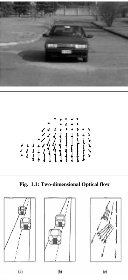
The optical flow is a velocity field in the image which transforms one image into the next image in a sequence. Optical flow is a vector field of pixel velocities based on the observable variations forms the time-varying image intensity pattern.

Fig. 1.1: Two-dimensional Optical flow

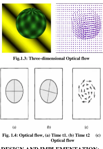
Fig.1.3: Three-dimensional Optical flow

Fig. 1.4: Optical flow, (a) Time t1. (b) Time t2 (c) Optical flow

2. DESIGN AND IMPLEMENTATION:

The Simulink model for this project mainly consists of three parts, which are “Velocity Estimation”, “Velocity Threshold Calculation” and “Object Boundary Box Determination”. For the velocity estimation, we use the optical flow block in the Simulink built in library. The optical flow block reads image intensity value and estimate the velocity of object motion using either the Horn-Schunck or the Lucas-Kanade.[4] The velocity estimation can be either between two images or between current frame and Nth frame back. We set N to be one in our model. After we obtain the velocity from the Optical Flow block, we need to calculate the velocity threshold in order to determine what is the minimum velocity magnitude corresponding to a moving object. To obtain this velocity threshold, we first pass the velocity through couple mean blocks and get the mean velocity value across frame and across time. After that, we do a comparison of the input velocity with mean velocity value. If the input velocity is greater than the mean value, it will be mapped to one and zero otherwise. The output of this comparison becomes a threshold intensity matrix, and we further pass this matrix to a median filter lock and closing block to remove noise. After we segment the moving object from the background of the image, we pass it to the blob analysis block in order to obtain the boundary box for the object and the corresponding box area. The blob analysis block in Simulink is very similar to the “regionprops” function in MATLAB. They both measure a set of properties for each connected object in an image file. The properties include area, centroid, bounding box, major and minor axis, orientation and so on. In this project, we utilize the area and bound box measurement. In our model, we only display boundary box that is greater than a certain size, and the size is determined according to the object to be track.[3]

3. METHODOLOGY:

The algorithm has following stages:

1) Firstly feed a video file to be tracked as an input.

2) Then convert color frames of video to grayscale video frames.

3) Next optical flow is computed between current frame and Nth frame back.

4) Then calculate velocity of motion vectors.

5) Out of all pixels of the frame only moving pixels are of moving object.

6) Compute magnitude of vector of velocity through optical flow & take a mean.

7) Median filter is used to get thresholded image of moving object.

8) Then blob analysis is performed on Thresolded image.

9) After that box can be drawn around that image.

10) Moving object tracked in that box by using bounding box and velocity is calculated by using formulas.

Fig 3.1(a): Original Video

Fig 3.1(c): Tracking the vehicle

3.1 Lucas-Kanade Algorithm:

The Lucas–Kanade method is a two-frame differential method for optical flow estimation developed by Bruce D. Lucas and Takeo Kanade.[6]

It introduces an additional term to the optical flow by assuming the flow to be constant in a local neighborhood around the central pixel under consideration at any given time.

The additional constraint needed for the estimation of the flow field is introduced in this method by assuming that the flow (V x, V y) is constant in a small window of size m X m with m > 1, which is centered at Pixel x, y and numbering the pixels within as 1...n, n = m2, a set of equations can be found:[7]

Where q1,q2,…qn are the pixels inside the window, and

are the partial derivatives of the image I

with respect to position x, y and time t, evaluated at the point and at the current time.

These equations can be written in matrix form Av=b, where

Fig.3.2: Simulink Block Diagram for Tracking Moving Objects Using Lucas-Kanade Algorithm

The Lucas-Kanade method obtains a compromise solution by the least squares principle. Namely, it solves the 2×2 system[8]

_{or where is the}

transpose of matrix A. That is, it computes

with the sums running from i=1 to n.

3.2 Horn-Schunck Algorithm:

The optical flow methods try to calculate the motion between two image frames which are taken at times t and t + δt at every pixel position. These methods are called differential since they are based on local Taylor series approximations of the image signal; that is, they use partial derivatives with respect to the spatial and temporal coordinates.[7]

Vip traffic.avi Image V:120X160, 15fps

RGB to intensity

Color space Conversion

Optical Flow Lucas Kanade )

Vec vel_th

I box

Image Draw

Rectangle

Pts.

Image To Video Display

To Video Display

Image

Image To Video Display

I

Image

Vel_values vel_lines

Images

Draw Lines

Pts.

Image

To Video Display Optical flow

on

Vel_threshold on

Original on

Optical flow lines

Motion Vector From Multimedia File

Threshold

Assume I (x, y, t) is the center pixel in a n×n neighborhood and moves by δx, δy in time δt to I (x+δx, y +δy, t+δt). Since I (x, y, t) and I (x + δx, y + δy,

t + δt) are the images of the same point (and therefore the

same) we have:

I (x, y, t) = I (x + δx, y + δy, t + δt) ………..(1)

Solving Eq (1) gives

………..(2)

Where, , , are intensity derivative in x, y ,t respectively and are the x and y components of the velocity or

optical flow of I (x, y, t).

Eq (2) is then solved us The Optical Flow block using the Horn – Schunck algorithm (1981) estimates the direction and speed of object motion from one video frame to another and returns a matrix of velocity component sing Horn-Schunck method.[6]

The Optical flow block using H-K algorithm estimates speed of Object motion from one video frame to another and returns a matrix of velocity components.

Thresholding returns a thresholded image differentiating the objects in motion(in white) and static background(in black).It is the process of assigning a label to every pixel in an image so that pixels with same label share same visual characteristics. [8]

A median filter is used to remove salt and pepper noise from thresholded image and eliminates intensity spikes without reducing sharpness of image.

In order to calculate velocity time of motion in seconds is t_ travelled = n/fps.

Velocity of vehicle in m/s is

Vel (m/s) = d _travelled(cm) / t_travelled

Fig. 3.3: Simulink Block Diagram for Tracking Moving Objects Using Horn-Schunck Algorithm

4. COMPARISON OF VARIOUS

ALGORITHMS:

Horn-Schunck is a global method that estimates flow everywhere.[7] Bt Lucas-Kanade algorithm is a local window based method that cannot solve for optical flow everywhere. Whenever noise is concerned, Lucas-Kanade algorithm is robust to noise in comparison to H-S algorithm. Average angular error is high in Horn-Schunck algorithm than Lucas-Kanade algorithm. There exist fast and accurate optical flow algorithms. Local and global methods can be combined for desired characteristics like dense flow estimate, make it robust to noise and Preserve discontinuities. Also the average angular error decreases by combining both algorithms. Horn-Schunck method Oversmooths the edges whereas Lucas-Kanade algorithm lacks smoothness.

The Horn-Schunck algorithm allows in general to move away from gradient flow.[8] The Horn-Schunck method is also very unstable in case of illumination artefacts in image sequences (due to the assumed brightness constancy). The Horn-Schunck algorithm was just the first algorithm for calculating optic flow; many others have been proposed since 1981, and motion analysis is still a very challenging subject in computer vision research.[9] Due to the aperture problem, results of the Horn-Schunck method correspond in general to gradient flow g

rather than to the correct 2D motion d at the given pixel.

We combine both local and global methods for the following requirements:

• Need dense flow estimate • Robust to noise

Vip traffic.avi

Image V:120X160, 15fps

RGB to intensity

Color space Conversion

Optical Flow (Horn-Schunc k)

Vec vel_th

I box

Image Draw Rectangle

Pts.

Image To Video Display

To Video Display

Image

Image To Video Display

I

Image

Vel_values vel_lines

Images Draw Lines

Pts.

Image

To Video Display Optical flow

on

Vel_threshold on

Original on

Optical flow lines

Motion Vector From Multimedia File

Threshold

• Preserve discontinuities

Below is shown a table illustrating Average angular error of various algorithms and sensitivity to noise in fig.4.1 & fig.4.2 respectively.

Table 4.1: Average angular error

Angular error Method

Average angular error

Lucas & Kanade

4.3

Horn & Schunck 9.8

Combining local and global

4.2

Fig 4.1: Average angular Error is more in Horn- Schunck than Lucas- Kanade

Fig 4.2 : Sensitivity to noise

PSNR of Lucas-Kanade algorithm is 32.09 and PSNR of Horn-Schunck algorithm is 30.71.So Signal to noise ratio of Lucas-Kanade algorithm is more than Horn-Schunck algorithm.[10]

Table 4.2: PSNR of various algorithms

Method PSNR

Lucas-Kanade algorithm 32.09

Horn-Schunck algorithm 30.71

5. CONCLUSION & FUTURE WORK:

6. REFERENCES

[1] A. M. Tekalp, E.F.(1995), “Digital Video Processing. Englewood Cliffs”, NJ: Prentice-Hall, 1995.

[2] “Different Approaches for Motion Estimation”, E.F.( 4th-6th June 2009 ), International Conference on control, automation, communication and energy conservation -2009.

[3] Chi-Cheng Cheng, and Hui-Ting Li .E.F.( 2006), “Feature-Based Optical Flow Computation”,

International Journal of Information

Technology,Vol.12,pp.7.

[4] Savan Chhaniyara, Pished Bunnun, Lakmal D. Seneviratne and Kaspar Althoefer, E.F.( MARCH 2008), “Optical Flow Algorithm for Velocity Estimation of Ground Vehicles: A Feasibility Study”, International Journal on smart sensing and intelligent systems, VOL. 1, pp. no. 1.

[5] E. Atkoˇci ¯unas, R. Blake, A. Juozapaviˇcius, M. Kazimianec., E.F.( 2005), “Image Processing in Road Traffic Analysis’. Nonlinear Analysis: Modelling and Control”, Vol. 10, No. 4, 315–332.

[6] S. Baker, I. Matthews, E.F.( March 2004 ), “Lucas-Kanade 20 Years On: A Unifying Framework”, IJCV, Vol.56, No. 3, ,pp. 221-255.

[7] B.K.P. Horn, B.G. Schunck, E.F.(1981),“Determining Optical Flow”, Artificial Intelligence, Vol. 2, pp. 185-203.

[8] P. Subashini, M.Krishnaveni, Vijay Singh, E.F.(August 2011), “Implementation of Object Tracking System Using Region Filtering Algorithm based on Simulink Block sets”, International Journal of Engineering Science and Technology(IJEST),Vol.3 No.8. PP-6744-6750.ISSN:0975-5462.

[9] J.L. Barron, D.J. Fleet, and S.S. Beauchemin, E.F.( February 1994 ), “Performance of Optical Flow Techniques”, International Journal of Computer Vision, , vol. 12(1), pp. 43-77.

[10]Bruhn, J. Weickert and C. Schnörr , E.F.(2005), “Lucas/Kanade meets Horn/Schunck: Combining local and global optic flow methods”, International Journal of Computer Vision, 61(3): 211–231.

[11]Bruhn, J. Weickert, C. Feddern, T. Kohlberger, C. Schnörr, E.F.(2003 - 2005 ), “Towards ultimate motion estimation: Combining highest accuracy with real-time performance”.

[12]Lazaros Grammatikopoulos, George Karras, Elli Petsa, E .F.( November, 2005 ),“Automatic Estimation of Vehicle, Speed from Uncalibrated Video Sequences”, International Symposium on Modern Technologies, Education & Professional Practice in Geodesy and related fields, Sofia,03 – 04.

[13]L. Li and Y. Yang:, E.F.(2010), “Optical flow estimation for a periodic image sequence”,IEEE Trans. on Image Processing, 19(1): 1-10.