Application of Graph Abstraction for
Performance Optimization of Wireless Ad Hoc
Networks: Two Node Scenarios
Md. Mohiuddin Khan
Department of Computer Science and Engineering Islamic University of Technology, Dhaka, Bangladesh
ABSTRACT
This paper examines the feasibility and efficiency of representation of wireless networks using graph abstractions. These abstractions represent wireless nodes and interactions between them as vertices and edges in a labelled graph. Vertices are defined with respect to different environmental and network protocol settings on a node while edges correspond to monitored performance metrics. In this paper we present the findings of the two node network. We use the upper layer metrics such as application layer goodput and fairness to characterize network performance. The parameters include network topologies as well as different traffic types and underlying transport protocols. Our results indicate that for many parameter settings of the vertices, the graph abstractions can be relatively simple. Each edge type can easily be modelled using basic mathematical functions. The results obtained from this simple scenarios work as a sanity check for larger networks.
General Terms
Wireless networks, Ad hoc networks
Keywords
Performance optimization, Network behavior
1.
INTRODUCTION
Recent times have seen an increasing deployment of wireless networks. Among the many factors contributing to this are the ease of set-up and maintenance, seamless access and availability of inexpensive hardware. However, the shared media for wireless communications presents new challenges, which were not present for fixed networks. One of those is the dependency of the wireless network performance on the operational environments, in addition to the classical dependency on the parameters of the protocol stack and the mixture of data flows.
The exhaustive study of the multitude of these dependencies is a NP-hard problem that cannot be addressed by a network simulator in any reasonable computing time. Therefore, we suggest applying graph abstractions to represent the wireless ad-hoc networks and find similarities between different wireless scenarios. As a result, one can limit the number of parameter permutations needed to be studied to characterize either a particular network scenario or a new network protocol.
In this paper, we systematically study how the network simulator, QualNet, reacts on parameter changes for small-scale wireless networks, and how those changes can be represented using graph abstractions.
The rest of the paper is structured as follows. In section 2, definition and terminology related to graphs and graph abstraction are discussed along with a summary on the related works on graph abstraction in wireless networks. Section 3 presents the proposed approach. Section 4 describes the simulation environment as well as the network scenarios, protocol and environmental parameters. Section 5 presents the results in detail while section 6 provides a detailed discussion on the results. Section 7 concludes the paper along with the proposal and outline for future work.
2.
DEFINITION AND RELATED WORK
2.1
Graphs and Graph Abstraction
Graphs are a special kind of data structure that can represent mathematical as well as real life problems. Structurally, a graph G is made up of a set of vertices V and a set of edges E. Pictorially these vertices are represented by points which are connected by lines which represent the corresponding edges. Edges and vertices can be labelled or named with numbers of alphabets. An edge of graph can also be assigned a number, called weight which may represent a particular property we are interested in, such as distances or costs. Graph coloring is one kind of graph labeling and it can refer to either vertex coloring or edge coloring. Generally, vertex/edge coloring means assigning labels (colors/values) to the vertices/edges so that no two adjacent vertices/edges have the same label.
With graph abstraction, the information available from a particular domain is represented with graphs; converting variables and values to corresponding vertices, edges, labels etc. As a result, the problem in hand reduces to a graph, providing computationally and often visually efficient expressions. The graphs then can be utilized to solve the problem.
2.2
Use of Graph Abstraction in Wireless
Networks
Nabeel et al. [3] provide hands-on insight to their previously published method of creating radio frequency (RF) maps for wireless local area networks (WLAN). Radio Frequency mapping is a technique to lessen the effect of interference in wireless network, which is prevalent now-a-days due to the availability and inexpensiveness of both access points and client devices. In the context of RF mapping, conflict graphs are directed graphs where the links of a network are represented by the nodes of the graph and there exists an edge between two nodes if they are interfering.
While determining upper and lower bounds of throughput for any given wireless network, Jain et al. [4] model the interference between neighboring nodes of the network with the help of conflict graphs. A similar representation of conflict graphs is also used by Liu et al. [5] in the context of increasing indoor wireless network capacity using directional antennas. In [6], Kodialam et al. represented the scheduling problem of a multi-hop wireless network with a graph edge-coloring problem. Nandagopal et al. [7] utilized graph abstraction to establish a framework for achieving MAC layer fairness in wireless networks.
3.
PROPOSED APPROACH
It is well understood that capturing the entirety of the environmental conditions, protocol parameters and interactions in wireless networks is a huge task. However,
often it is not always necessary to work with highly precise models, lower level of precision suffices while giving considerable gains in time and computational resources. For
example instead of performing all possible simulations to study the behavior of the network, one can generalize and classify the probable scenarios so that the number of scenarios that have to be studied decreases effectively. Graphs can be used to achieve this goal.
Graphs are often used to represent wired networks whereas wireless networks are typically described and displayed using spatial point distribution [8, 9]. We suggest using graphs to represent wireless networks, similar to the literature reviewed in the preceding subsection. In addition to represent the nodes in a network with graph vertices, we also propose to color (i.e. to label) the edges between the nodes according to the dependency of the performance on the distance and individual protocol settings. Each of the colors would represent a range of distance in which the network shows similar behavior. In our thesis we evaluated our approach on small networks and check on the number of colors that one may need to use. The composite graph abstraction includes several layers. The first layer corresponds to the interference graph [4] where the number of labels depends on (a) achieved throughput and (b) defines if nodes are within the sensing range of each other. The next layers correspond to different individual protocol settings, (see Figure 1). The superposition of different graph abstractions allows to more accurately model wireless networks and therefore, as we see in the next chapters, explains its performance.
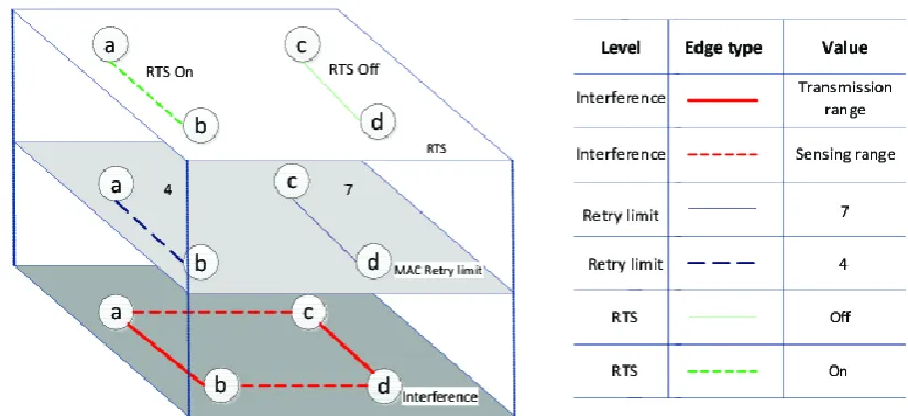
[image:2.595.90.503.467.656.2]In Figure 1, we have shown a pictorial depiction of the graph abstractions. Here, the graph represents a network consisting of four nodes with particular MAC layer setting under study. For the interference subgraph we can see that the node pairs a-b and c-d can only are in transmission range, while a-c and a- b-d can only sense each other. The MAC retry limit layer shows the individual settings on the nodes. In this work we assume that both nodes involved into a connection have the same MAC setting, which, in general, might not be true and would require a larger pool of labels. The superposition of all these layers containing relevant information builds the resulting graph abstraction representing the entire network.
Fig 1. Graphs as the superposition of different protocol layers
4.
SIMULATION
SETUP
AND
SCENARIO DESCRIPTION
4.1
Simulator
We have used QualNet [10] as the simulator in our thesis. QualNet is a state-of-the-art commercial networks simulator capable of providing a comprehensive framework for
modelling, creating, analyzing and verifying network protocols and architectures. Besides the default build of the software, custom interfaces were also used, mainly to access the simulation results in real-time.
statistics. Hence, we have used MATLAB1 to run QualNet simulation and collect statistics during the runtime.
4.2
Choice of Traffic
Application layer itself poses a number of parameters to play with. The choice of application type to simulate is not a trivial task as the subset of applications we choose should be representative either for the realistic environment or reflect the diverse behavior of the network. For our simulation scenarios, we have picked the following three types of traffic:
CBR: Communicated with UDP, representing connectionless communication
FTP: Communicated with TCP, representing reliable communication
VoIP: Representing IP telephony
Thus, we believe our choice of these three types of traffic signifies the general spectrum of usage in typical scenarios.
4.3
Scenario
[image:3.595.327.529.99.196.2]In this paper, we have investigated small ad hoc networks consisting of two nodes for the application of graph abstraction. This is a simple network where the two nodes act as senders and receivers without the presence of any additional interference. This results in a graph with two nodes. The two nodes communicate with each other with no other interfering nodes, as shown in Figure 2. The motivation here is to observe the performance in this basic scenario and finding out possible patterns in performance metrics in relation with the distance between nodes.
Fig 2. Simple two node scenario
4.4
Setup and Method
Simulating large networks (or a portion of it) is a complex task. In the seminal paper, Floyed et al. [11] described the relevant problems. They have explained that it is obvious that exploring the entire parameter space is rarely feasible. They have said "the challenge is to figure out which parameters to modify, and in what combinations." We have adopted the approach introduced by them – we simulated a scenario for different values of a particular parameter while keeping all the other parameters fixed. In this way, we can monitor the effect of that particular parameter on the performance.
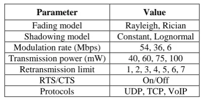
In Table 1, we have summarized the parameters which we have monitored throughout the thesis. These parameters include environmental conditions (shadowing and fading models), physical layer entities (modulation rate, transmission power), link layer entities (retransmission limit, RTS/CTS), transport layer entities (TCP Segment size) and application layer entities (FTP, CBR, VoIP). These parameters span across the entire protocol stack and can be combined to observe the cross-layer effects on performance.
1
[image:3.595.341.514.262.372.2]MATLAB is a product of MathWorks Inc. Version 7.11.0.584 (R2010b) was used in our work.
Table 1. Observed parameters and their corresponding values
Parameter Value
Fading model Rayleigh, Rician Shadowing model Constant, Lognormal Modulation rate (Mbps) 54, 36, 6 Transmission power (mW) 40, 60, 75, 100
Retransmission limit 1, 2, 3, 4, 5, 6, 7
RTS/CTS On/Off
Protocols UDP, TCP, VoIP
Some of the important fixed parameters are listed in Table 2. These are among the parameters that remain constant throughout the various scenarios.
Table 2. Some of the fixed parameters
Parameter Value
MAC type 802.11a
Pathloss model Two-ray ground Antenna model Omnidirectional Antenna height 1.5 meter
CWmin 15
CWmax 1031
SIFS 16
sTCP variant Reno
In QualNet, UDP is implemented with setting up a constant bit rate (CBR) application in the particular node; generating an array of 1450 byte size packets with an interval of 0.4 ms. Similar packet size and interval rate is used in case of simulating TCP flows. VoIP was simulated with an average talk time of one minute.
4.5
Performance Metrics
For measuring the performance, throughput is the obvious choice for UDP and TCP. When a scenario has contending flows, we also measure the fairness of the flows. To measure fairness, we have used Jain's fairness index [12], which can be obtained by:
2 2.
=
i i
x
N
x
FI
where
N
is the number of competing entities andx
i is therespective share of entity
i
among them. Though fairness is not applicable to the scope of the current paper as we are dealing with only a single flow, it will be useful for larger scenarios with three, four or more nodes.For measuring VoIP output, we have used MOS (Mean Opinion Score) which is a recognized method for subjective determination of transmission quality [13]. MOS is measured in a forward scale of 0 (worst) to 5 (best). It is mentionable that in QualNet, the highest value of MOS in wireless domain does not go above 3.3.
4.6
Sensing Range
[image:3.595.67.269.412.479.2]scenarios, one has to analyze the effect of RTS/CTS with the introduction of the hidden terminal. The propagation threshold in QualNet wireless transmission is set to-75 dBm. Signals below this value are not delivered to the destination.
5.
RESULTS
In the previous section, we have discussed about the simulation environment and the parameters that we would used in our simulations. In this section, we put those settings into use by simulation the two node scenario. The rest of this section presents the results obtained from the two-node scenario. At first we discuss the effect of the environmental settings such as shadowing and fading, then working our way up the protocol stack including modulation rate, transmission power and retry limit. In the end, we talk about the effect of the different types of traffic that run on top of TCP or UDP transport protocols.
5.1
Shadowing
[image:4.595.335.544.76.219.2]Having conducted the default scenario with lognormal shadowing, we opt for constant shadowing for comparing effects of the difference of shadowing model on the throughput. In both cases the shadowing mean is set to 4, which is the default value.
Fig 3. Throughput vs. distance for shadowing models
As shown in Figure 3, with constant shadowing the effective distance in which the connection maintains a high throughput is increased. In fact, the graph clearly depicts that with constant shadowing, a linear shift is added to that of lognormal shadowing. In case of lognormal shadowing we see the throughput starts to decline at thirty meters of distance and gradually goes down to zero at around forty meters. With constant shadowing, we see the same behavior - throughput starts to fall down at forty meters and becomes zero at around sixty meters.
5.2
Fading
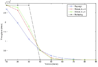
In default case, a QualNet simulation is conducted with no fading. To represent commonly observed fading effects concerning whether a line-of-sight signal is present or not, we conduct experiments with the fading model set to Rayleigh [14] and Rician [15]. In case of Rician model, the fading max velocity is kept to 10 meters/sec and the K-factor value is set to 4 and 6 to see the effect of the difference. In total, we have four scenarios representing the four different fading models. Each of these four scenarios are simulated both with lognormal and constant shadowing.
Fig 4. Throughput vs distance for different fading models
Figure 4 shows the results obtained for the four scenarios with the lognormal shadowing. As we can observe, the fading models incorporate a sense of gradualism in the declining behavior of throughput with respect to the distance.
Keeping in mind that Rayleigh fading is actually a specialized case of Rician fading (with K = 0), we can see that the we have no fading and Rayleigh fading a the two extremes of the behavior and Rician models with varying K-factors in the middle. With constant shadowing, we see a similar behavior as that of lognormal shadowing, only with the added shift in distance discussed in the previous section.
5.3
Modulation Rate
In Figure 5 we can see the throughput of the connection for three different modulation rates. We have chosen 54Mbps, 36Mbps and 6Mbps to represent the highest, mid-range and lowest modulation rates among the available options in 802.11a. Expectedly, with the increasing modulation rate, the throughput tends to fall down more sharply with increasing distance.
[image:4.595.71.273.339.478.2]By default, the scenarios are conducted with RTS/CTS turned off and with lognormal shadowing. In these conditions, each of the modulation rates shows a symmetric behavior - keeping a constant throughput for a particular distance and then getting lower in a linear way before it goes down to zero with the nodes getting completely out of the communicating range.
Fig 5. Throughput vs. distance for modulation rates
5.4
Transmission Power
[image:4.595.330.531.556.694.2]resulting behavior is plotted in Figure 6. As we are dealing with a two-node scenario with no outside interference, the sole effect that we observe is an increase of the transmission range with the increasing transmission power.
Fig 6. Throughput vs. distance for transmission powers
5.5
Retry Limit
[image:5.595.69.263.127.248.2]Retry limit is a 802.11 MAC protocol parameter that decides how many times a packet will be retransmitted by the sender before it is discarded. There are two types of retry limits - station short retry count (SSRC) and station long retry count (SLRC). Each station maintains two of these retry limits for packets under and over the RTS/CTS threshold, respectively. As we conducted our two node scenario with RTS/CTS turned off, all the transmitted packets indeed are shorter than the threshold. So, we vary the SSRC from 1 to 7 and observe the corresponding throughput.
Fig 7. Throughput vs distance for different retry limits
We observed that there is no change in the throughput for varying retry limits while the two nodes are within 30 meters of distance. As we see in a zoomed out version of the plot in Figure 7, the throughputs do vary while the nodes are 40 meters apart. We see that with retry limit as low as 1, we get higher throughput than when the limit is 6 or 7. The throughputs for 2, 3, 4 and 5 retries lie in between the two extremes. It is evident from the results that throughput decreases with the increasing number of retransmissions as it slow down the link. However, the amount of lost packets in this scenario is not high so retransmission limit does not have a significant impact.
5.6
TCP Segment Size
We simulate TCP among the two nodes for observing the behavior of the nodes for reliable data transmission. The data rate and default parameters are the same as those described in
case of UDP traffic. The important TCP parameters used in the QualNet configuration files is listed in Table 3.
Table 3. TCP parameters for two-node TCP Scenario
Parameter Value
TCP variant RENO Delaying ACK packets Yes
TCP send buffer 30720 bytes TCP receive 30720 bytes
In case of TCP, we observe the throughput for three different TCP segment size. In the default scenario, the TCP maximum segment size (MSS) is set to 1500 bytes. As we are using 1450 bytes packets, in this case there was only one TCP segment. We set two other segment size limits, namely 500 bytes and 750 bytes, resulting in 3 and 2 TCP segments for each application layer packets.
[image:5.595.328.530.413.547.2]We can see the throughput for the corresponding segment sizes in Figure 8. Understandably, the throughput goes down as the segment per packet increases; as a result of the overhead incurred by the increasing number of segments. In case of no fragmentation we have a throughput of 23.6 Mbps whereas it goes down to 15.5 Mbps for the MSS of 750 bytes, decreasing 34.2%. For the MSS of 500 bytes, we have a throughput of 11.7 Mbps, which is half of the throughput with no fragmentation. Moreover, with segmentations increasing, we see a slower degradation in throughput and emergence of non-linear behavior as the distance increases.
Fig 8. Throughput vs distance for different TCP MSS
5.7
VoIP
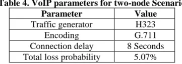
[image:5.595.68.266.414.539.2] [image:5.595.337.518.670.734.2]Voice over Internet Protocol (VoIP) [16] is one of the most widely used communication medium now-a-days. Using VoIP through wireless networks is a popular choice. Hence, we simulate VoIP traffic in our two node scenario. The relevant VoIP parameters used in the QualNet simulation are listed in Table 4.
Table 4. VoIP parameters for two-node Scenario Parameter Value
Traffic generator H323 Encoding G.711 Connection delay 8 Seconds Total loss probability 5.07%
observed for both UDP and TCP, the MOS keeps steady up to a certain distance and declines afterwards. With lognormal shadowing, we get a MOS of 3.30 for distances up to thirty meters. Following the ITU-T recommendation in [13], this falls between Good (4) and Fair(3).
5.8
Mixed Traffic
In this section, we present the results while the sender node sends a mixture of traffic to the receiver. For simplicity, we have only considered uni-directional cases, thus keeping the sender (node 1) and receiver (node 2) fixed. We also observe the behavior when one of the flows is given precedence over the other and the other way around.
5.8.1
UDP and TCP
In this case, node 1 sends both TCP and UDP traffic to node 2. With both TCP and UDP having the same priority, we observe that the TCP flow is completely dominated by the UDP flow, as shown in Figure 9.
Same Precedence
TCP higher Precedence
Fig 9.Throughput for TCP and UDP mixed traffic with different precedence
However, when having precedence over UDP, TCP enjoys higher throughput while the UDP throughput goes down to around fifty percent of the original value but do not die completely like TCP; as depicted in Figure 9.
5.8.2
UDP and VoIP
When we send both UDP and VoIP application traffic from node 1 to node 2, we observe that UDP throughput is not affected by the VoIP traffic. This is probably due to that fact that the VoIP flow is too weak a flow to disrupt the UDP connection.
On the other hand, we also do not see any decrease in VoIP MOS with the presence of the UDP traffic. These behavior
corresponds to that describe in [17], as they show that VoIP does have adverse effect on UDP traffic but effective when we have a large number of VoIP connection in the network.
5.8.3
TCP and VoIP
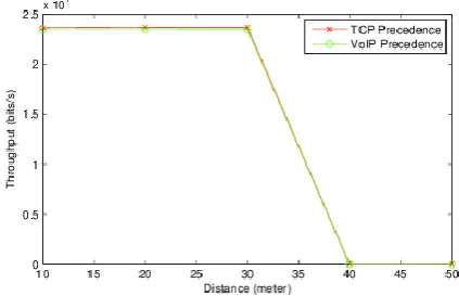
[image:6.595.329.541.233.375.2]With an added TCP connection between the two nodes, we observe the VoIP MOS to get as low as 1. TCP's reliable delivery nature is the factor behind this behavior, described in detail by Wang et al. [18]. However, as we provide higher priority to the VoIP flow over the TCP flow, the MOS of the VoIP flow goes high up to 3.30. This performance gain in VoIP does not cost TCP any performance degradation, as shown in Figure 10. This behavior also conforms to those described in [18].
Fig 10. TCP throughput with VoIP
6.
DISCUSSION
As the previous sections containing the resulting graphs from the two node scenario shows, four distinctly behaving zones are visible in them. In the first zone the throughput (or MOS in case of VoIP) remains constant, starts to go down in the second zone, in zone three it reaches (close to) zero where the nodes can only sense each other and in the fourth zone the nodes are completely out of range from each other. For the two nodes scenario in these chapter we have showed the first three zones. These zones are speculated based upon the distance between the two nodes. Hence, we can represent this zonal behavior in the realm of graph abstraction by differing colors. As shown in Figure 11, the link color will be determined by the distance and hence will represent the zonal behavior. This, in turn will provide a graph abstraction.
The fact to note here is that, we are not running real life experiments rather conducting the scenarios in simulation environment. However, with the objective to reduce the number of simulations required to predict the behavior of an ad hoc wireless network, we have seen that for various different parameters there are zones inside which the behavior is predictable.
[image:6.595.70.270.286.573.2] [image:6.595.316.544.644.746.2]The performed experiments indicate a linear performance degradation in the second zone for most of the observed parameters. The exception of this trend is visible in case of different fading models (Figure 4) and transmission power levels (Figure 6). With the changes in fading models, the graphs changed their behavior significantly. As seen in case of Rayleigh fading, we see the straight line behavior gives way to a much smoother curve like behavior.
For the majority of the parameters that we have observed, the effect on the performance can be described by the following equation:
else 0
if < if
= = e
Performanc bx c A x D
A x a
x f
Where is the distance between sender and receiver, and are constants, A and D are distance boundaries. The behavior of the Rayleigh and Rician fading models (Figure 4) can be best fitted with a third degree polynomial,
[image:7.595.336.508.72.349.2] [image:7.595.84.252.208.249.2], or an exponential equation,
Table 5.
Fitting coefficients and error measures for Rician fading model graph
Measure Exponential Cubic
a 5.27e+007
b -0.04628
p 55.28
q -53.78
r -8.748e+005
s 4.043e+007
R-square 0.8911 0.9482
Table 6.
Fitting coefficients and error measures for Rician fading model graph
Measure Exponential Cubic
a 4.73e+007
b -0.05149
p -54.14
q 1.+004
r -1.371e+006
s 3.99e+007
R-square 0.9802 0.9953
The coefficients along with the R-squared values are listed in Table 5 and 6. The corresponding fitting graphs are shown in Figure 12. From the values shown in the table it seems that for Rician model, exponential function is a lesser fit than the cubic one. However, if we exclude the first point (at 10 meters distance), the R-square value for the exponential fit reaches to 0.9643, which is higher than the cubic fit. The corresponding values of a and b in that case becomes 1.275e+008 and -0.07397.
Rician
[image:7.595.75.259.353.442.2]Raleigh
Fig 12. Cubic and exponential fitting models for Rician and Rayleigh fading
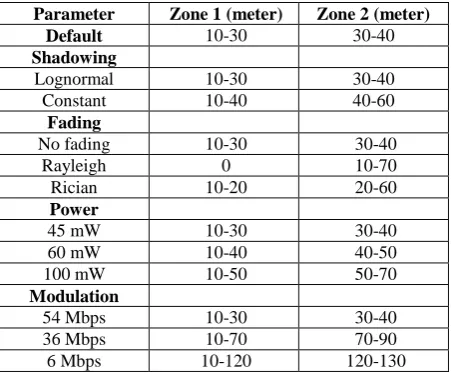
In Table 7, the two zones of distances for the various parameters are summarized.
Table 7. Summary of distance zones for the scenario
Parameter Zone 1 (meter) Zone 2 (meter) Default 10-30 30-40
Shadowing
Lognormal 10-30 30-40
Constant 10-40 40-60
Fading
No fading 10-30 30-40
Rayleigh 0 10-70
Rician 10-20 20-60
Power
45 mW 10-30 30-40
60 mW 10-40 40-50
100 mW 10-50 50-70
Modulation
54 Mbps 10-30 30-40
36 Mbps 10-70 70-90
6 Mbps 10-120 120-130
[image:7.595.316.542.438.625.2] [image:7.595.79.257.482.571.2]7.
CONCLUSION AND FUTURE WORK
While simulating this simple two node scenario, our main focus was on the independent tuning of some of the network parameters without any consideration on the cross-layer aspect. As a result, we get a simple and clear indication of the effect of the parameters on the network output. This showed us what parameters will be important to observe in real scenarios. This simple scenario also works as a sanity check for the more complex three to four node scenarios. We were able to identify and pinpoint the zonal behavior of the network and presented the throughput vs. distance ratio for various selected important parameters.We are currently working on larger scenarios involving three and four nodes where we will implement the knowlede and observations we gained from the basic two node scenario. In case of those larger networks, obviously one has to deal with issues like fairness and contention, hidden terminal, orientation of nodes etc. The data, observation and simulations presented in this paper can work as a stepping stone of the future research work involving ad hoc networks - both in simulations and testbeds.
8.
REFERENCES
[1] M. Garetto, J. Shi, and E. Knightly, “Modeling media access in embedded two flow topologies of multi-hop wireless networks,” in Proceedings of the 11th annual international conference on Mobile computing and networking, p. 214, ACM, 2005.
[2] S. Razak, V. Kolar, and N. B. Abu-Ghazaleh, “Modeling and analysis of two-flow interactions in wireless networks,” Ad Hoc Networks, vol. 8, no. 6, pp. 564 – 581, 2010.
[3] N. Ahmed, U. Ismail, S. Keshav, and K. Papagiannaki, “Online estimation of RF interference,” in CoNEXT ’08: Proceedings of the 2008 ACM CoNEXT Conference, (New York, NY, USA), pp. 1–12, ACM, 2008.
[4] K. Jain, J. Padhye, V. N. Padmanabhan, and L. Qiu, “Impact of interference on multi-hop wireless network performance,” Wirel. Netw., vol. 11, no. 4, pp. 471–487, 2005.
[5] X. Liu, A. Sheth, M. Kaminsky, K. Papagiannaki, S. Seshan, and P. Steenkiste, “Dirc: increasing indoor wireless capacity using directional antennas,” SIG-COMM Comput. Commun. Rev., vol. 39, pp. 171–182, August 2009.
[6] M. Kodialam and T. Nandagopal, “Characterizing achievable rates in multi-hop wireless networks: the joint routing and scheduling problem,” in Proceedings of the 9th annual international conference on Mobile computing and networking, Mobi-Com ’03, (New York, NY, USA), pp. 42–54, ACM, 2003.
[7] T. Nandagopal, T.-E. Kim, X. Gao, and V. Bharghavan, “Achieving mac layer fair-ness in wireless packet networks,” in Proceedings of the 6th annual international con-ference on Mobile computing and networking, MobiCom ’00, (New York, NY, USA), pp. 87–98, ACM, 2000.
[8] J. Riihijarvi, P. Mahonen, and M. Rubsamen, “Characterizing wireless networks by spatial correlations,” Communications Letters, IEEE, vol. 11, no. 1, pp. 37 –39, 2007.
[9] G. Resta and P. Santi, “An analysis of the node spatial distribution of the random waypoint mobility model for ad hoc networks,” in Proceedings of the second ACM international workshop on Principles of mobile computing, POMC ’02, (New York, NY, USA), pp. 44– 50, ACM, 2002.
[10]“Qualnet network simulator.” Website, October 2012. http://qualnet.com/
[11]S. Floyd and V. Paxson, “Difficulties in simulating the internet,” IEEE/ACM Trans. Netw., vol. 9, pp. 392–403, August 2001.
[12]R. Jain, D.-M. Chiu, and W. Hawe, “A quantitative measure of fairness and dis-crimination for resource allocation in shared systems,” tech. rep., Digital Equip-ment Corporation, Technical Report DEC-TR-301, September 1984.
[13]“P.800 : Methods for subjective determination of transmission quality.” Website, November 2010. http://www.itu.int/rec/T-REC-P.800-199608-I/en.
[14]B. Sklar, “Rayleigh fading channels in mobile digital communication systems characterization,” Communications Magazine, IEEE, vol. 35, pp. 90 –100, July 1997.
[15]C. Loo and N. Secord, “Computer models for fading channels with applications to digital transmission,” Vehicular Technology, IEEE Transactions on, vol. 40, pp. 700–707, Nov. 1991.
[16]B. Goode, “Voice over internet protocol (voip),” Proceedings of the IEEE, vol. 90, pp. 1495 – 1517, September 2002.
[17]S. Garg and M. Kappes, “An experimental study of throughput for udp and voip traffic in ieee 802.11b networks,” in Wireless Communications and Networking, 2003. WCNC 2003. 2003 IEEE, vol. 3, pp. 1748 –1753 vol.3, 2003.