Munich Personal RePEc Archive
A note on the double k-class estimator in
simultaneous equations
Lahiri, Kajal and Gao, Chuanming
2002
A Note on the Double
k-class Estimator in
Simultaneous Equations
Chuanming Gao, Kajal Lahiri
∗Department of Economics, State University of New York at Albany, Albany, NY 12222
ABSTRACT
Dwivedi and Srivastava (1984, DS) studied the exact finite sample prop-erties of Nagar’s (1962) double k-class estimator as continuous functions of its two characterizing scalars k1 and k2, and provided guidelines for their
choice in empirical work. In this note we show that the empirical guidelines provided by DS are not entirely valid since they did not explore the com-plete range of the relevant parameter space in their numerical evaluations. Wefind that the optimal values ofk2 leading to unbiased and mean squared
error (MSE) minimizing double k-class estimators are not symmetric with respect to the sign of the productρω12, whereρis the correlation coefficient
between the structural and reduced form errors, and w12 is the covariance
between the unrestricted reduced form errors. Specifically, whenρω12is
pos-itive, the optimal value of k2 is generally positive and greater thank1, which
partly explains the superior performance of Zellner’s (1998) Bayesian Method of Moments (BMOM) and Extended MELO estimators reported in Tsurumi (1990).
JEL classification: C30
Keywords: Limited Information, Simultaneous Equations, Finite Sample,
Mean Squared Error.
*Corresponding author. Tel: (518) 442 4758; fax: (518) 442 4736; e-mail: [email protected].
1
Introduction
In an important paper, Dwivedi and Srivastava (1984, hereafter DS) studied
the exactfinite sample properties of Nagar’s (1962) doublek-class estimator. After deriving thefirst two moments of the estimator as continuous functions of the two characterizing scalarsk1 andk2, they found that k2 can be chosen
such that a double k-class estimator is unbiased for a givenk1. DS also
ana-lyzed a result originally derived by Srivastava, Agnihotri and Dwivedi (1980)
that it is always possible to choose k2 such that a double k-class
estima-tor has smaller mean squared error (MSE) than that of a k-class estimator.
Through some numerical evaluations, DS provided guidelines on the choices of k1 andk2 for empirical work. They found that the value ofk2 which
char-acterizes an unbiased doublek-class estimator for a givenk1 between−1and
1 is smaller than the value of k1 and declines as the prespecified value of k1
increases. Most of the time, this value of k2 was found to be negative. They
also concluded that the MSE minimizing value of k∗
is negative in majority of the cases and is larger in absolute value than the associated value of k1.1
The main purpose of this note is to show that the empirical guidelines
provided by DS are not entirely valid since they did not explore the whole range of the relevant parameter space in their numerical evaluations. DS
adopted their model specifications from Sawa (1972) that were originally used to study the properties of single k-class estimators. We find that the optimal values ofk2 leading to unbiased and MSE minimizing doublek-class
estimators are not symmetric with respect to the sign of the product ρω12,
1See also Srivastava (1990) for a comprehensive survey on the properties of double
whereρ is the correlation between the disturbances of the structural and the
reduced form equations, and ω12 is the covariance between the unrestricted
reduced form errors. For the single k-class estimator this asymmetry is not an issue. In all the specifications considered by DS, the implied value of ρ
is −0.514 and ρω12 is always negative. In addition we also derive a simple
expression for the optimal value of k2 such that a double k-class estimator
has the smallest MSE for a given k1. Wefind that when ρω12 is positive, the
optimal value of k2 is generally positive and greater than k1.
2
Finite sample moments
Using the notations in DS, let us consider the following structural model:
y1 =βy2+X1γ+u, (1)
wherey1 andy2 areT×1vectors of observations on the included endogenous
variables;X1 is aT×lmatrix of observations onl(<Λ) exogenous variables;
u is a T ×1vector of disturbances with zero mean and finite variance of σ2
. It is assumed that the structural equation is identified and the reduced form of the system is written as
( y1 y2 ) =X1( π11 π21 ) +X2( π12 π22 ) + ( v1 v2 ), (2)
where X = ( X1 X2 ) is a T ×Λ matrix with full column rank of
obser-vations on Λ exogenous variables in the system with X0
1X2 = 0. The rows
of ( v1 v2 ) are assumed to be independently and identically distributed as
N(0, Ω), whereΩis pds andΩ=
Ã
ω11 ω12 ω21 ω22
!
A double k-class estimator for the structural coefficient β, with
charac-terizing scalars k1 andk2, can be expressed as
b
βDKC =βbKC + (k1−k2)(y02Ay2)− 1
y0
2P y1, (3)
where βbKC is the k-class estimator of β with characterizing scalar k1,
P =I−X(X0X)−1
X0 =I−X1(X0 1X1)−
1
X0
1−X2(X20X2)− 1
X0 2, and
A= (1−k1)[I−X1(X10X1)− 1
X0
1] +k1X2(X20X2)− 1
X0 2.
We also define the following:
m = 1
2(T −l), n= 1
2(T −Λ), δ = 1
2ω22π022X20X2π22, and for non-negative
integers a,b, c, and d,
φ(a;b) = e−δ
∞ X
j=0
Γ(m−n+j−a)
Γ(m−n+j+b) ·
δj
j!, (4)
ψd(a;b;c)
−1≤k1<1
=e−δ
∞ X α=0 ∞ X j=0
(dα+ 1)kα1
Γ(m+j−a−1)Γ(n+α+b)
Γ(m+j +α+c)Γ(n) ·
δj
j!. (5)
DS obtained the exact analytical expressions for mean and MSE of the
double k-class estimator of β. When −1 ≤ k1 <1 and2m ≥1, the bias of
the double k-class estimator of β is given by
E(βbDKC)−β= (β−
ω12 ω22
)(δψ0(1; 0; 1)−1) + (k1−k2) ω12 ω22
ψ0(1; 1; 1). (6)
When−1≤k1 <1and 2m ≥3, the MSE of the double k-class estimator of
β is given by
E(βbDKC −β)2
= (β− ω12
ω22
)2
+ (k1−k2) 2
(ω12
ω22
)2
ψ1(1; 2; 2)
+ω11.2 2ω22
[(1−k2) 2
ψ1(0; 1; 1) + (m−n)ψ1(0; 0; 1) +δψ1(1; 0; 2)]
+δ(β− ω12
ω22
)2
[1
2ψ1(0; 0; 1) +δψ1(1; 0; 2)−2ψ0(1; 0; 1)]
+2ω12
ω22
(β− ω12
ω22
where ω11.2 =ω11−ω 2
12/ω22. The bias and MSE are similarly defined when
k1 is set at unity.
From (6) and (7), DS derived two interesting results. First, for a given
k1, the doublek-class estimator is unbiased if the value of k2 is set as
ku = k1+ ω22 ω12
(β− ω12
ω22
)[δψ0(1; 0; 1)−1
ψ0(1; 1; 1)
] if −1≤k1 <1, (8)
= 1 +ω22
ω12
(β− ω12
ω22
)[δφ(0; 1)−1
nφ(1; 0) ] if k1 = 1. (9)
Second, the MSE of the double k-class estimator is less than that of k -class estimator with −1 ≤ k1 < 1 if the value of k2 is between k1 and k∗,
with k∗ de
fined as
k∗
= k1+{[(1−k1) ω11.2
ω22
ψ1(0; 1; 1)
+2ω12
ω22
(β− ω12
ω22
)[δψ1(1; 1; 2)−ψ0(1; 1; 1)]]
/[(ω12
ω22
)2
ψ1(1; 2; 2) + ω11.2
2ω22
ψ1(0; 1; 1)]}, (10)
If k1 = 1,
k∗ = 1 +{[ω12 ω22
(β−ω12
ω22
)(δφ(1; 1)−φ(1; 0))]
/[ω11.2 2ω22
φ(2; 0) + (n+ 1)(ω12
ω22
)2
φ(1; 0)]}. (11)
Using (7), we furtherfind that for a givenk1, the value of k2 that results
in the double k-class estimator with the minimum MSE is given by
k∗∗
= 1
2(k1+k
∗
). (12)
Even though (12) was not explicitly derived in DS, the above expression for the optimalk2 is not surprising since the MSE of doublek-class estimator is
3
Numerical evaluations
In order to get a feel about the magnitude and even the signs of ku and
k∗, DS tabulated the values of k
u and k∗ for selected values of k1 and δ
(k1 = 0,±0.2,±0.6,±1 and δ = 1,10,25,50,100). Following Sawa (1972)
and Srivastava et al.(1980), Dwivedi and Srivastava (1984) set
β = 1, ω12
ω22
= 0.4, ω11.2
ω22
= 1, (13)
and considered the following three cases:
Case I. Λ= 5, l = 2, and T = 10,20,30,50
Case II. Λ= 10, l= 3, and T = 20,30,50
Case III.Λ = 15,l = 5, andT = 20,30,50
For the sake of brevity, we only report results which corresponds to Case III in DS (i.e., Λ = 15, l = 5) with T = 50.2 Our Specification 1 has the same setup as in DS, and we try to duplicate the tabulated values of ku and
k∗ in DS. In this speci
fication, as in all the specifications considered by DS, the implied value of ρ is -0.514 and ρω12/ω22 = −0.2056.3 Since ω22 > 0,
the implied ρω12 is always negative in their setup. We then consider several
alternative values of the parameters defined in (13) to demonstrate our point. In Specification 2, we set β =−1, other parameters being the same. These parameter values implyρ= 0.814 andρω12/ω22= 0.3256.In Specification 3,
we setω12/ω22 =−0.4,other things being the same as in Specification 1. This
leads to an implied ρvalue of -0.814 andρω12/ω22= 0.3256. In Specification
2Numerical calculations are done using GAUSS for Windows Version 3.2.35 on a
Pen-tium II 450MHz PC.
3ρ is derived using the following relationships: β−ω
12/ω22 = −ρ p
σ2/ω 22, and
σ2/ω
4, we further set ω12/ω22 = 1.6 yielding ρ = 0.514 and ρω12/ω22 = 0.8224.
The results from our numerical evaluations are collected in Tables 1, 2 and 3. We will first discuss results in Tables 1 and 2.
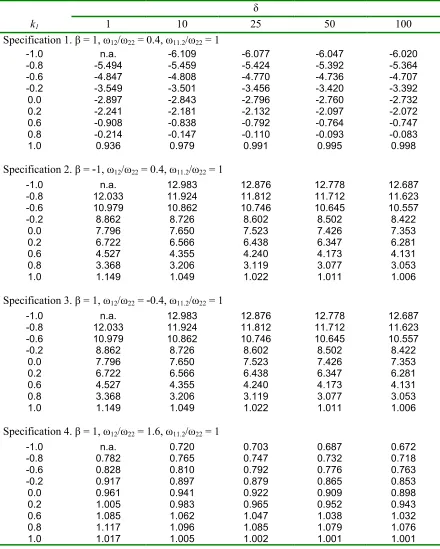
Based on our extensive experiments with the specifications considered in DS, we found that there are substantial computational errors in the numerical evaluations reported by DS. In their Table 1 reporting values of ku, only the
results when δ = 1 and 10 have acceptable levels of accuracy. As δ gets larger (viz. δ= 25, 50,100), their results became increasingly imprecise, and clearly unacceptable. This is seen if one compares ku values in their Table 1
(last panel of Case III, m = 22.5, n= 17.5) with those in our Table 1 (first panel). More strikingly, the values ofk∗ reported in Table 2 of DS seem to be
erroneous for all values of δ they considered. This is revealed by comparing the k∗ values in their Table 2 (last panel of Case III, m = 22.5, n = 17.5)
with those in our Table 2 (first panel). For instance, DS reported that for our Specification 1, whenk1 = 0,δ = 100, the value ofk∗ is−1071.807, while
it is −2.732 according to our calculation.
Overall we find that the value of k∗ is of the similar magnitude as k
u.
It does not exhibit the tremendous variation as reported in DS. Also as a result of improved precision in our calculations, we find that the value of ku
changes monotonically as δ increases for a given −1< k1 <1. Interestingly,
when k1 is set equal to 1, wefind that the value of ku is independent of δ.4
Results from Specification 2 show that the optimal values ofkuandk∗may
be all positive and greater than k1, invalidating the major conclusion in DS
4We had difficulty in obtaining reliable results for specifications with k
1 =−1when
that they take large negative values for most of the time and are less thank2.
These results may be easily explained by (6) and (7). First let us consider the determinants of the bias for the double k-class estimator. Observe thatβbKC
is biased in the direction ofρ, as noted by Mariano (1982). Negativeρimplies
a downward bias, positive ρ implies an upward bias in βbKC. Since for the
single k-class estimatork2 =k1, thefirst term(β−ω12/ω22)(δψ0(1; 0; 1)−1)
in (6) represents the bias of βbKC, and is of the same sign as that of ρ. In order to reduce the bias of the double k-class estimator, the second term
(k1 −k2)(ω12/ω22)ψ0(1; 1; 1) in (6) should have sign opposite to that of ρ.
Since ψ0(1; 1; 1)>0, we require (k1−k2)ω12 to be of the opposite sign ofρ.
Therefore when ρω12 < 0, i.e., ρ and ω12 are of opposite signs, the value of
ku should be less than k1, as observed by DS. However when ρω12 > 0, the
value of ku should be greater than k1, as shown in our Specification 2.
The dependence of the value of k∗ on the sign of ρω
12 can be explained
in a similar way. The first four terms in (7) do not depend on the sign of
ρ or ω12 explicitly. Regarding the last term in (7), note that [δψ1(1; 1; 2)− ψ0(1; 1; 1)] is negative and does not change sign for the wide range of values
of δ considered. Thus, in order to make MSE of the doublek-class estimator for a prespecifiedk1to be less than that ofβbKC, we should choose the value of
k2 such that (ω12/ω22)(β−ω12/ω22)(k1−k2)is negative. Therefore the value
of k∗ should be selected in a similar way as for the value ofk
u,depending on
the sign of ρω12.
Note that the optimal values of ku (Table 1) and k∗ (Table 2) under
opposite signs, leaving ρω12/ω22 = 0.3256 in both cases. It implies that ku
andk∗ are symmetric with respect to the signs of (ω
12, ρ). The results from
Specification 4 show that both ku and k∗ move towards 1 as k1 approaches
1. Again from Specifications 3 and 4, we find that the optimal values of ku
andk∗ are greater than k
1 when ρω12 >0, but less than k1 whenρω12 <0.
Table 3 does not have a counterpart in DS and reports the optimal values
of k2 (k∗∗) and the resulting mean squared errors (MSEs) of the double
k-class estimator with characterizing scalars k1 and k∗∗. Comparing MSE
figures under Specifications 2 and 3, we again find that they are symmetric with respect to the signs of (ω12, ρ). It is shown that the values of k∗∗ are
much closer toku than tok∗, suggesting that unbiasedness is the dominating
criterion in fixing the MSE-minimizing value of k2. When the value of k1 is
set at 1, the value of k∗∗ is very close or equal to 1.
4
Conclusions
There has been a renewed interest in studying the properties of double k -class estimators. For instance, Zellner (1986, 1998) has shown that the
ex-tended minimum expected loss (ZEM) and the Bayesian Method of Moments (BMOM) estimators can be conveniently evaluated as doublek-class
estima-tors where the values of the two characterizing scalarsk1andk2 are uniquely
determined by elegant balanced loss functions involving both ‘goodness offit’ and ‘precision of estimation’ criteria. An attractive feature of BMOM
of the likelihood function is unknown.5 Tsurumi (1990) compared a number
of Sampling theory and Bayesian estimators, and found that ZEM generally outperforms others, and is certainly among the top three in all cases.
Based on finite sample expressions for the first two moments of double
k-class estimators, Dwivedi and Srivastava (1984) concluded that for a given value of k1, the value of k2 that yields unbiased and minimum MSE double
k-class estimator is smaller than k1, and is generally negative. We find that
their guidelines on the choice ofk1andk2 are not entirely valid, and could be
misleading. In their numerical evaluations they did not consider an important
segment of the relevant parameter space. We point out that unlike the single
k-class estimator, the properties of the double k-class estimator are severely
affected by the signs of ρ and ω12. The optimal value of k2 for a given k1
will be quite different depending on the sign of the product ofρand ω12. DS
inadvertently considered only cases whereρω12 <0, and found correctly that
optimal values of k2 should be less than the value of k1. We, however, show
that if ρω12 > 0, the optimal values of k2 should be greater than k1 and is
generally positive. By comparing the optimal values of ku and k∗∗, we also
find that the unbiasedness criterion dominates in determining the optimal value of k2.
5In a recent paper Zellner and Tobias (2001) extend previous BMOM results to show
References
Dwivedi, T.D, and V.K. Srivastava (1984). Exact finite sample proper-ties of double k-class estimators in simultaneous equations. Journal of
Econometrics 25, 263-283.
Mariano, R.S. (1982). Analytical small-sample distribution theory in econo-metrics: the simultaneous-equation case. International Economic Re-view 23, 503-533.
Nagar, A.L. (1962). Double k-class estimators of parameters in simulta-neous equations and their small sample properties. International
Eco-nomic Review 3, 168-188.
Sawa, T. (1972). Finite-sample properties of the k-class estimators.
Econo-metrica 40, 653-680.
Srivastava, V.K. (1990). Developments in double k-class estimators of pa-rameters in structural equations. In: Carter, R.A.L., Dutta, J. and Ullah, A., eds.,Contributions to Econometric Theory and Application,
Essays in honour of A.L. Nagar (Springer-Verlag).
Srivastava, V.K., B.S. Agnihotri and T.D. Dwivedi (1980). Dominance of double k-class estimators in simultaneous equations. Annals of
Insti-tute of Statistical Mathematics 32, 387-392.
Srivastava, V.K., T.D. Dwivedi, M. Belinsky and R. Tiwari (1980). A nu-merical comparison of exact, large-sample and small-disturbance ap-proximations of properties of k-class estimators. International
Eco-nomic Review 21, 249-252.
Tsurumi, H. (1990). Comparing Bayesian and non-Bayesian limited infor-mation estimators. In: Geisser, S., Hodges, J.S., Press, S.J., Zellner, A., eds.,Bayesian and Likelihood Methods in Statistics and Economet-rics (North-Holland, Amsterdam).
Zellner, A. (1986). Further results on Bayesian minimum expected loss (MELO) estimates and posterior distributions for structural coeffi -cients. In: Slottje, D., eds., Advances in Econometrics, Vol. 5, pp. 171-182.
Zellner, A. (1998). The finite sample properties of simultaneous equations’ estimates and estimators: Bayesian and non-Bayesian approaches.
Zellner, A. and J. Tobias (2001). Further results on Bayesian Method of Moments analysis of the multiple regression model. International
Table 1. Values of k2 (ku) leading to an unbiased double k-class estimator
δ
k1 1 10 25 50 100
Specification 1. β = 1, ω12/ω22 = 0.4, ω11.2/ω22 = 1
-1.0 n.a. -4.419 -4.401 -4.385 -4.370
-0.8 -3.935 -3.917 -3.898 -3.882 -3.868
-0.6 -3.433 -3.414 -3.395 -3.379 -3.365
-0.2 -2.429 -2.407 -2.388 -2.373 -2.361
0.0 -1.925 -1.903 -1.883 -1.869 -1.858
0.2 -1.420 -1.397 -1.378 -1.365 -1.356
0.6 -0.404 -0.380 -0.364 -0.355 -0.350
0.8 0.112 0.134 0.145 0.150 0.154
1.0 0.657 0.657 0.657 0.657 0.657
Specification 2. β = -1, ω12/ω22 = 0.4, ω11.2/ω22 = 1
-1.0 n.a. 6.979 6.936 6.898 6.862
-0.8 6.516 6.473 6.430 6.392 6.358
-0.6 6.011 5.966 5.923 5.885 5.853
-0.2 5.000 4.950 4.905 4.870 4.842
0.0 4.492 4.439 4.395 4.361 4.336
0.2 3.981 3.926 3.882 3.852 3.830
0.6 2.944 2.886 2.850 2.829 2.816
0.8 2.404 2.354 2.328 2.316 2.308
1.0 1.800 1.800 1.800 1.800 1.800
Specification 3. β = 1, ω12/ω22 = -0.4, ω11.2/ω22 = 1
-1.0 n.a. 6.979 6.936 6.898 6.862
-0.8 6.516 6.473 6.430 6.392 6.358
-0.6 6.011 5.966 5.923 5.885 5.853
-0.2 5.000 4.950 4.905 4.870 4.842
0.0 4.492 4.439 4.395 4.361 4.336
0.2 3.981 3.926 3.882 3.852 3.830
0.6 2.944 2.886 2.850 2.829 2.816
0.8 2.404 2.354 2.328 2.316 2.308
1.0 1.800 1.800 1.800 1.800 1.800
Specification 4. β = 1, ω12/ω22 = 1.6, ω11.2/ω22 = 1
-1.0 n.a. -0.145 -0.150 -0.154 -0.158
-0.8 -0.016 -0.021 -0.025 -0.029 -0.033
-0.6 0.108 0.104 0.099 0.095 0.091
-0.2 0.357 0.352 0.347 0.343 0.340
0.0 0.481 0.476 0.471 0.467 0.465
0.2 0.605 0.599 0.595 0.591 0.589
0.6 0.851 0.845 0.841 0.839 0.837
0.8 0.972 0.966 0.964 0.962 0.962
Table 2. Values of k*
δ
k1 1 10 25 50 100
Specification 1. β = 1, ω12/ω22 = 0.4, ω11.2/ω22 = 1
-1.0 n.a. -6.109 -6.077 -6.047 -6.020
-0.8 -5.494 -5.459 -5.424 -5.392 -5.364
-0.6 -4.847 -4.808 -4.770 -4.736 -4.707
-0.2 -3.549 -3.501 -3.456 -3.420 -3.392
0.0 -2.897 -2.843 -2.796 -2.760 -2.732
0.2 -2.241 -2.181 -2.132 -2.097 -2.072
0.6 -0.908 -0.838 -0.792 -0.764 -0.747
0.8 -0.214 -0.147 -0.110 -0.093 -0.083
1.0 0.936 0.979 0.991 0.995 0.998
Specification 2. β = -1, ω12/ω22 = 0.4, ω11.2/ω22 = 1
-1.0 n.a. 12.983 12.876 12.778 12.687
-0.8 12.033 11.924 11.812 11.712 11.623
-0.6 10.979 10.862 10.746 10.645 10.557
-0.2 8.862 8.726 8.602 8.502 8.422
0.0 7.796 7.650 7.523 7.426 7.353
0.2 6.722 6.566 6.438 6.347 6.281
0.6 4.527 4.355 4.240 4.173 4.131
0.8 3.368 3.206 3.119 3.077 3.053
1.0 1.149 1.049 1.022 1.011 1.006
Specification 3. β = 1, ω12/ω22 = -0.4, ω11.2/ω22 = 1
-1.0 n.a. 12.983 12.876 12.778 12.687
-0.8 12.033 11.924 11.812 11.712 11.623
-0.6 10.979 10.862 10.746 10.645 10.557
-0.2 8.862 8.726 8.602 8.502 8.422
0.0 7.796 7.650 7.523 7.426 7.353
0.2 6.722 6.566 6.438 6.347 6.281
0.6 4.527 4.355 4.240 4.173 4.131
0.8 3.368 3.206 3.119 3.077 3.053
1.0 1.149 1.049 1.022 1.011 1.006
Specification 4. β = 1, ω12/ω22 = 1.6, ω11.2/ω22 = 1
-1.0 n.a. 0.720 0.703 0.687 0.672
-0.8 0.782 0.765 0.747 0.732 0.718
-0.6 0.828 0.810 0.792 0.776 0.763
-0.2 0.917 0.897 0.879 0.865 0.853
0.0 0.961 0.941 0.922 0.909 0.898
0.2 1.005 0.983 0.965 0.952 0.943
0.6 1.085 1.062 1.047 1.038 1.032
0.8 1.117 1.096 1.085 1.079 1.076
Table 3. Values of k2 (k**) with Minimum MSEs in parentheses
δ
k1 1 10 25 50 100
Specification 1. β = 1, ω12/ω22 = 0.4, ω11.2/ω22 = 1
-1.0 n.a. -3.555 (0.094) -3.538 (0.057) -3.524 (0.031) -3.510 (0.015) -0.8 -3.147 (0.136) -3.130 (0.090) -3.112 (0.053) -3.096 (0.029) -3.082 (0.013) -0.6 -2.724 (0.135) -2.704 (0.086) -2.685 (0.050) -2.668 (0.026) -2.654 (0.012) -0.2 -1.875 (0.130) -1.850 (0.077) -1.828 (0.042) -1.810 (0.021) -1.796 (0.010) 0.0 -1.448 (0.128) -1.421 (0.072) -1.398 (0.037) -1.380 (0.019) -1.366 (0.009) 0.2 -1.021 (0.125) -0.991 (0.066) -0.966 (0.033) -0.949 (0.017) -0.936 (0.008) 0.6 -0.154 (0.121) -0.119 (0.054) -0.096 (0.026) -0.082 (0.014) -0.074 (0.007) 0.8 0.293 (0.127) 0.327 (0.051) 0.345 (0.024) 0.354 (0.013) 0.359 (0.007) 1.0 0.968 (0.314) 0.990 (0.075) 0.995 (0.029) 0.998 (0.014) 0.999 (0.007)
Specification 2. β = -1, ω12/ω22 = 0.4, ω11.2/ω22 = 1
-1.0 n.a. 5.992 (0.119) 5.938 (0.073) 5.889 (0.042) 5.844 (0.021)
-0.8 5.617 (0.176) 5.562 (0.117) 5.506 (0.071) 5.456 (0.040) 5.411 (0.020) -0.6 5.190 (0.179) 5.131 (0.115) 5.073 (0.068) 5.022 (0.037) 4.979 (0.018) -0.2 4.331 (0.187) 4.263 (0.111) 4.201 (0.062) 4.151 (0.033) 4.111 (0.017) 0.0 3.898 (0.194) 3.825 (0.109) 3.761 (0.059) 3.713 (0.032) 3.676 (0.016) 0.2 3.461 (0.204) 3.383 (0.108) 3.319 (0.056) 3.273 (0.030) 3.240 (0.015) 0.6 2.563 (0.253) 2.477 (0.110) 2.420 (0.053) 2.387 (0.028) 2.366 (0.014) 0.8 2.084 (0.325) 2.003 (0.119) 1.960 (0.055) 1.938 (0.029) 1.926 (0.015) 1.0 1.075 (1.249) 1.024 (0.238) 1.011 (0.080) 1.006 (0.035) 1.003 (0.016)
Specification 3. β = 1, ω12/ω22 = -0.4, ω11.2/ω22 = 1
-1.0 n.a. 5.992 (0.119) 5.938 (0.073) 5.889 (0.042) 5.844 (0.021)
-0.8 5.617 (0.176) 5.562 (0.117) 5.506 (0.071) 5.456 (0.040) 5.411 (0.020) -0.6 5.190 (0.179) 5.131 (0.115) 5.073 (0.068) 5.022 (0.037) 4.979 (0.018) -0.2 4.331 (0.187) 4.263 (0.111) 4.201 (0.062) 4.151 (0.033) 4.111 (0.017) 0.0 3.898 (0.194) 3.825 (0.109) 3.761 (0.059) 3.713 (0.032) 3.676 (0.016) 0.2 3.461 (0.204) 3.383 (0.108) 3.319 (0.056) 3.273 (0.030) 3.240 (0.015) 0.6 2.563 (0.253) 2.477 (0.110) 2.420 (0.053) 2.387 (0.028) 2.366 (0.014) 0.8 2.084 (0.325) 2.003 (0.119) 1.960 (0.055) 1.938 (0.029) 1.926 (0.015) 1.0 1.075 (1.249) 1.024 (0.238) 1.011 (0.080) 1.006 (0.035) 1.003 (0.016)
Specification 4. β = 1, ω12/ω22 = 1.6, ω11.2/ω22 = 1