A Novel Design Method of Two Stage CMOS Operational Transconductance Amplifier used for Wireless Sensor Receiver

(1)

A Novel Design Method of Two-stage CMOS

Operational Transconductance Amplifier used for

Wireless Sensor Receiver

Radwene Laajimi

Nawfil Gueddah

Mohamed Masmoudi

ABSTRACT

Operational transconductance amplifier (OTA) is one of the most significant building-blocks in integrated discret-time filters used in analog to digital converter (ADC) for Sigma-delta converter. In this paper we designed a novel design method of two-stage CMOS amplifier in AMS 0.35μm technology. P-Spice simulation results confirm the proposed OTA circuit. In fact, we achieved a gain band width (GBW) equal to 55 MHz, Cut-off frequency of 85 KHz and 57 dB gain (Av). In addition our new method allowed us to reduce settling time (St) to 15.6 ns and a slew rate (SR) of 0.1 V/µs at ±1.5V supply voltage. Eventually we have also succeeded in reducing the average power consumption to 1.65 mW while driving 3 pF load capacitor.

General Terms

Microelectronic Components Circuits Devices & Systems

Keywords

Wireless sensor, Operational amplifier, CMOS OTA Design.

1. INTRODUCTION

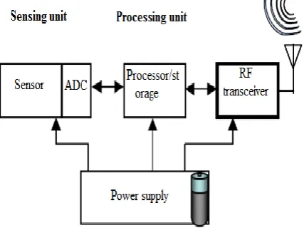
[image:1.595.62.276.551.711.2]

In the last few years, wireless sensor networks [1-2] (WSNs) have increased rapidly and become one of the most interesting areas of research [3]. It is composed of a number of wireless sensor nodes which form a sensor field and a sink. To ensure high performance of these large numbers of nodes they require low-cost, low-power, and capacity of communication at short distances in order to perform limited computation and communicate wirelessly in the WSNs [4-5].

Fig. 1: Block diagram of a sensor node

Many applications are included in industrial and home automation, medical monitoring, automatic meter reading, alarms and agriculture. The fig. 1 shows the block diagram of a sensor node.

It is composed of four blocks: power supply, communication, processing unit, and sensors.

The power supply block has the purpose to power the node and usually consists of a battery. The communication block is an RF transceiver to provide a bidirectional wireless communication channel.

The processing unit is composed of an internal memory to store data, applications programs, and a microcontroller unit (MCU) to process data. The sensing unit block links the sensor node to the physical world and transmits a signal to Analog-to-Digital Converter (ADC) [6].

The paper is organized as follows.

Section II presents the conventional two-Stage operational amplifier transconductance (OTA) used for wireless sensor receiver. In section III the design of Modified tow Stage Miller OTA circuit with cascode current source is presented. Modified two-stage Miller OTA with designed current source is presented in section IV, while their full comparison is given in section V in which the performance of each OTA is indicated in table 9. Conclusion is drawn in Section VI.

1.1 Receiver architectures

The main objective of a receiver for wireless communication applications is to recover the base band signals that are modulated on a carrier wave at radio frequencies. The design of a high performance, low power integrated radio frequency receiver in mainstream silicon technologies CMOS is a very challenging task involving numerous tradeoffs during the design process, especially between noise, linearity and power consumption. In this paper we introduce with a description of the direct conversion receiver or homodyne which is the most widely used receiver architecture for highly integrated and low-power consumption. This receiver architecture directly down converts the signal to base band rather than converting it into an intermediate frequency (IF) first, and image rejection is no longer necessary in this approach. The block diagram of a direct conversion or homodyne architecture is illustrated in fig. 2.

(2)

International Journal of Computer Applications (0975 – 8887) Volume 39– No.11, February 2012

The frequency translation is performed by using two mixers using 0° and 90° phase shifted local oscillator (LO) signals. Finally, the I and Q base band signals are amplified and low pass filtered before the analogue to digital converter (A/D) conversion is intervened.

[image:2.595.55.284.127.339.2]

Fig. 2: Block diagram of a direct conversion or homodyne architecture

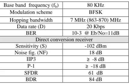
To achieve the objective cited above, all aspects of the receiver [7] and radio system need to be addressed as shown in table 1. (Base band, Modulation scheme, hopping bandwidth, data rate, Sensitivity, Noise fig., IIP3, P-1, SFDR, BDR...).

Table 1 : Sensor receiver specifications Base band frequency (fb) 80 KHz

Modulation scheme BFSK Hopping bandwidth 7 MHz (863-870) MHz

Data rate (D) 20 Kbps BER 10-3 @ Eb/No=11dB

Direct conversion receiver Sensitivity (S) -102 dBm Noise fig. (NF) 18 dB

IIP3 ≥ -8 dB

P-1 ≥ -18 dB

SFDR 61 dB

BDR 84 dB

To characterise the sensor thermal noise (Nt) is given by:

dB

f

N

_t





174 

10 log

₁₀

(

_b

)





125

Another two elements defining sensor are SNRin, SNRout (Signal to Noise Ratio) which are based on the following formula:

dB

N

S

SNR

in





t



23 dB

D

f

N

E

SNR

b

dB b

out

10 log

10

5

0































As shown in fig. 3, (Eb /N0 ) is equal to 11 with Noncoherent Frequency Shift Keying ̎ NC -BFSK ̎ to attenuate a bit error rate (BER) of 10-3 which is based on the following formula:

o N

b E

BFSK

NC

e

BER

2

1

2

1



[image:2.595.319.570.157.433.2]







Fig. 3: Bit error rate (BER) for BPSK, C-BFSK and NC-BFSK

The Noise fig. is defined as:

dB

SNR

dB

SNR

NF

_in _out

out in

18 )

(

)

(





The effective number of bits of sigma-delta (Neff) converter is given by [21]:



 



 



2 2L 1 2L



2

eff log 2N 1 2L 1 OSR π

2 1

N    

Where N represents number of bits of the quantization circuitry (N = 1), L represents order of modulator (L = 1) and OSR means Over Sampling Ratio which is based on the following formula:

b s

f

F

OSR





2

[image:2.595.60.275.456.596.2]

(3)

1.2 Sigma-Delta analog to digital converter

(ADC)

Sigma-Delta (εΔ) analog to digital converters (ADC) have been successful in realizing high resolution consumer. (εΔ) converters are well suited for low bandwidth, high-resolution acquisition, and low cost, making them a good ADC choice for many applications such as wireless sensor. As shown in fig. 4, Sigma-delta converters combine an analog sigma delta modulator with a more complex digital filter. Accuracy depends on the noise and linearity performance of the modulator, which uses high performance operational amplifiers transconductance.

The operational transconductance amplifier (OTA) is an important component for various analog circuits and systems. It is widely used as active element in variablegain amplifiers, data converters, interface circuits, continuous time oscillators, switched capacitor filters and sample and hold circuits. Depending on system needs, OTA circuit with high open loop gain, high slew rate and large bandwidth is highly desired. The high slew rate and bandwidth ensure a small settling time, whereas the high gain improves the settling accuracy. For this reason we design here a novel design technique of (OTA).

Delta Sigma

Modulator

Digital Low

Pass Filter

Analog signal in

Digital signal out

Fig. 4 : Block diagram of the A/D converter On the one hand, dynamic range is defined as [8]:





























N _L L

dB

OSR

L

DR

₂

1 2 2

10

1

2

1

2

3 log

10

On the other hand, the dynamic range of an nb-bit Nyquist rate ADC is given by [9]:

76 .

1

02 .

6 





n

b

DR

For an 8-Bit ADC the dynamic range from the above formula is 49.92 dB. Oversampling ratio (OSR) to achieve DR = 49.92 dB is calculated to be 59.96. To simplify the decimator design, the oversampling ratio is usually chosen in powers of 2 and hence 64 has been chosen as the oversampling ratio which is indicated in the previous paragraph.

2. CONVENTIONAL TWO-STAGE

CMOS OTA

[image:3.595.322.542.112.232.2]

2.1 Design and performance

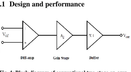
Fig. 4: Block diagram of conventional two-stage op-amp with output buffer

In order to have high performance ADC and switched capacitor filters, we need OTAs which have both high (DC) gain and a high gain bandwidth product (GBW) [10].

Generally, Operational amplifiers (op-amp) have sufficiently high voltage gain so that when the negative feedback is applied, the closed-loop transfer function can be made practically independent of the gain of the op-amp. This principle is employed in many useful analog circuits and systems. The primary requirement of an op-amp is to have an open loop gain which is sufficiently large to implement the negative feedback concept. One of the popular op-amp is a two-stage Miller op-amp shown in fig. 4. This last is made up of three stages even though it is often referred to as a “two-stage” op-amp, ignoring the buffer stage. The latter introduces an important concept of compensation. The primary goal of compensation is to maintain stability when negative feedback is applied around the operational amplifier.

(4)

A A B B C C D D E E F F G G H H I I J J 1 1 2 2 3 3 4 4 5 5 6 6

7 Page: 1 of 1 Size: A No: 7

Rev: 31 07-Dec-2011 09:04 Created: 10-Nov-2011

[image:4.595.57.279.74.391.2]

File: C:\Users\radwene\Desktop\Modif_Article_2012\miller_____ota.sch M8 M5 M6 M1 M2 M4 M7 M3 Cc Cl Vdd Vss Ibias

Fig. 5: Two-Stage Miller OTA [12]

2.2 Theoretical study

Fig.6 : Small signal equivalent circuit for two-stage op-amp

As shown in fig. 6, we present the small equivalent circuit in order to focus on the input differential stage.

We obtain a differential gain (Av1) of stage 1:

               4 2 5 5 1 1 4 2 2 1 . 1 . 1 2 . . 2 ' L V L V I I L W Kp g g g V V A En Ep ds ds m in out v

Gain of stage 2 is:

























7 6 6 6 7 7 6 7 7 2

.

1 .

1

2 .

.

2 L

V

L

V

I

L

W

Kn

g

A

En Ep ds ds m v

The overall gain of the amplifier is

A

_v



A

_v₁

.

A

_v₂ The gain bandwidth is:

c m

C

g

GBW

.

2

1





Where gm1 is the transconductance of M1, gds = parameter transconductance drain to source

According to [13] we use the following formula:

A

v

≥ 682.66

q

A

_v



2 

1

1 A

v

≥ 56.6 dB

Where q is the quantum of the Sigma-Delta ADC which is expressed as:

0029

.

0

2 )]

5 .

1 (

5 .

1 [

2

10







V

Full_Nscale

q

In this case we assume the overall gain Av more than 57 dB and to ensure good stability op-amp phase margin should be also more than 60 degree.

In [15], It is mentioned that GBW ≥ 3 Fs, but in this work it is recommended to have GBW more than 50 MHz in order to apply the following formula [14]:

b v

f

A

GBW





Where:

MHz

KHz

f

A

_v



_b



682 .

66 

80 

54 .

6 GBW



54 .

6 MHz

fb is the base band frequency and Av is the overall gain. All of op-amp has a restriction on its operating voltage range, CMR limits (Common input Mode Range) is the border of the scale range of each input op-amp, outside these limits cause output distortion. CMR can be presented by:

1 1 5 5 5 5

/

.

/

.

2 L

W

Kp

I

L

W

Kp

I

V

CMR

_



_DD



_TP



3 3 5

/

.

W

L

Kn

I

V

CMR

_



_SS



_TP



_Tn



In fig. 4, two-stage op-amp transconductance can be analyzed as follows:

6 6 6

/

.

2 L

W

Kp

I

V

OUT

_



_DD



7 7 6

/

.

2 L

W

Kn

I

V

OUT

_



_SS



2

2 1 ss

I

ID



;

c

C

I

SR

rate

slew

₍

₎



5

(5)

According to [15], we can propose a simple method based on gm/ID to determine (W/L) for each transistor of amp-op, because most methods for analytical synthesis of analog circuits suppose that the MOS transistors are either in strong inversion or in weak inversion. Our proposed methodology allows a unified synthesis methodology in all regions of MOS transistor.

The design procedure is illustrated as follows:

First of all, it is necessary to choose the value of the compensation capacitor Cc. For 60° phase margin, we use the following relationship:

Cc > 0.22×CL Cc=1 pF

Then the value of the bias current (Ibias) is determined based on the slew rate requirements: Ibias= 330µA. From Vgd3 = 0, transistor M3 is in saturation. Since the systematic offset condition provides that the drain voltage of M4 is equal to the drain voltage of M3.

The systematic offset condition makes the drain voltage of M1 equal to the drain voltage of M2. Consequently the condition for M2 being saturated is the same as the condition for M1 being saturated. We have Vgd8 = 0 thus transistor M8 is always in saturation. Transistors M5 and M6 form a current mirror with transistor M8.

In this case, we consider that the transistors have the same length (L= 1µm) to conserve symmetry and matching for all transistors, we require that:

W1=W2, W3=W4, W5=W8

Thus I1, I5 and I7 can be expressed as follows:

bias

I

L

W

L

W

I

.

/

8 8

5 5

5















;

I

bias

L

W

L

W

I

.

/

8 8

6 6

7















bias

I

L

W

L

W

I

_















8 8

5 5 5

1

/

2

1

2

2.3 Technological specification

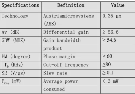
[image:5.595.314.545.69.226.2]

In order to realize a low power and low noise op-amp transconductance amplifier this is the most significant building-blocks in integrated discrete-time filters use for Sigma-delta analog to digital converter (Wireless Sensor Receiver). We must respond to technological specifications and requirements listed in Table 2.

Table 2 : Op Amp specifications

Specifications Definition Value

Technology Austriamicrosystems (AMS)

0.35 µm

Av (dB) Differential gain ≥ 56.6 GBW (MHZ) Gain bandwidth

product

≥ 54.6

PM (degree) Phase margin ≥ 60

fb (KHz) Cut-off frequency ≥80

SR (V/µs) Slew rate ≥ 0.1

Pmoy (mW) Average power

consumed

< 3 mW

V_dd(V) Positive power source

+1.5

Vss (V) Negative power

source

-1.5

CL (pF) Output load

capacitance

3

CC (pF) Compensation

capacitance

1

Vout (V) Output-voltage swing -1.2V to

1.2V

2.4 Op-Amp simulation

Referring to fig. 5 and respecting the specifications and the requirements shown in table 2, the size of different devices are calculated. Table 3 presents the parameters values of op-amp miller OTA. By using Pspice, we proceed to simulate the circuit given by fig. 5. We determine various characteristics such as gain, phase margin, power consumption, noise, slew rate, and offset.

Table 3 :Op Amp parameters values

Devices Value

M1, M2 W=24µm L=1µm M3, M4 W=10µm L=1µm M5, M8 W=41µm L=1µm

M6 W=220µm L=1µm

M7 W=148µm L=1µm

Supply voltage Vdd=1,5V Vss= -1,5V

Load capacitance Cl = 3pF

Compensation capacitance Cc = 1 pF

Bias current 350µA

2.4.1 Frequency open loop analysis

100 1k 10k 100k 1M 10M 100M

Frequency (Hz)

-100 -50 0 50

V

o

lt

a

ge

M

a

gn

it

u

de

(

d

B

),

P

h

ase

(d

eg

[image:5.595.50.246.412.497.2]

)

Fig. 7 : Simulated transfer function of amplifier Magnitude (dB) and phase (degree) of the Basic Two-Stage

Miller OTA

[image:5.595.53.281.609.768.2]

(6)

2.4.2 Unity feedback analysis

20 30 40 50 60 70 80 90

Time (ns) -1.0

-0.5 0.0 0.5

V

o

ut

(

V

),

'

V

(N

p)

'

()

(32.45n, 382.33m) (26.16n, -912.71m) dx=-6.29n dy=-1.30 m=205.93M

µs

V

dt

V

d

SR



(

out

)



₀

_.

₂

_/

V

out

V

in

Fig. 8 : Step transient response showing the slew

-As shown in fig. 8, a step is applied from -1V to 0.6 V at the input with unity feedback configuration. As was measured, the amplifier’s slew rate is 0.2 V/µs for the rising edge.

20 30 40 50 60 70 80 90

Time (ns)

-1.0 -0.5 0.0 0.5

'V

in

'

V

ou

t'

(

V

ol

t) _{Settling time}

S

t

= 17 ns

Fig. 9 : Step transient response showing the settling time of the Two-Stage Miller OTA

-The unity gain configuration is also used for settling time and peak over shoot measurement. This is the length of time for the output voltage of an op amp to approach. It remains within, a certain tolerance of its final value. The settling time equal to 17 ns is presented in fig. 9.

[image:6.595.319.546.74.354.2]

The output swing measured peak to peak shown in Fig. 10 is found to be -1.375 V to 1.375 V.

Fig. 10 : Transient Response showing the swing of 2.75 V of the OTA

2.4.3 DC sweep analysis

-0.005 0.000 0.005 0.010

Vin (V)

-1.5 -1.0 -0.5 0.0 0.5 1.0 1.5

V

o

ut

(

V

)

[image:6.595.62.286.102.252.2]

Input OffsetVoltage = 0.5 mV

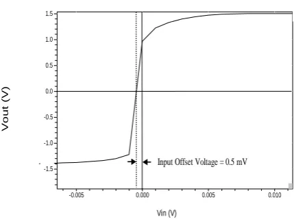
Fig. 11 : Transfer characteristics showing the input offset voltage of the of the Two-Stage Miller OTA

Fig. 11, shows the transfer characteristics obtained from DC sweep analysis. The input offset voltage is approximately calculated as 0.5 mV.

2.4.4 Summary table

[image:6.595.54.275.311.460.2] [image:6.595.321.536.424.584.2]

(7)

[image:7.595.378.486.74.240.2]

Table 4 : Summarizes the simulation results of the of the Basic Two-Stage Miller OTA

Parameters

Value

Slew rate (SR) 0.2 V/µs

DC Offset 0.5 mV

Gain 57 dB

Gain bandwidth (GBW) 59 MHz

Cut-off frequency (fb) 90 KHz

Phase margin (PM) 68 °

Average power consumed 3.5 mW Output-voltage swing -1.3 to 1.1 Supply voltage ±1.5V Settling time (St) 16 ns

3. MODIFIED TWO-STAGE MILLER

OTA CIRCUIT WITH CASCODE

CURRENT SOURCE

3.1 Analyses and specifications

In this paper, we proposed a modified OTA in which bias circuit was actively designed by NMOS transistors. For completeness, we first, analyzed and implement a Basic two-stage Miller OTA to prove the efficiency of the proposed design OTA.

In Fig. 12, the bias circuit consisted of NMOS cascode current source which is formed of five transistors (M9, M10, M11, M12, M13).

A B C D E F G H I J

1 1

2 2

3 3

4 4

5 5

6 6

M8

M5 M6

M1 M2

M4 M7

M3

Cc Cl Vdd

Vss M9

M10

M11

M13

[image:7.595.60.294.432.670.2]

M12

Fig. 12 : Modified Two-Stage Miller OTA with cascode current mirror

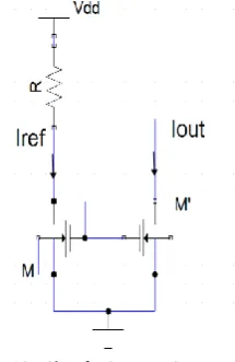
On the one hand, current source is one of the basic building blocks of analog VLSI systems. For low voltage design circuit, current source has to be with low input and output voltages. The accuracy and output impedance are the most important parameter to determine the performance of the current source. The basic simple current source with NMOS transistors (M, M’) is shown in fig. 13.

Fig. 13 : Simple Current Source

On the other hand, the basic current source needs to be stabilized over a large output voltage range, a high output impedance current source might needed. This is accomplished by putting two current sources in “cascade” to each other. The most popular current source circuit known as the cascode current source is shown in Fig. 14. Here, cascode current mirror can be used for the duplication of current Iref to provide higher output resistance and lower symmetric error. The NMOS cascode mirror consists of four transistors (M10, M11, M12, M13). It has high output impedance, and provides a low systematic transfer error.

It is well known that CMOS active resistors are very important blocks in VLSI analog designs, mainly used to replace the large value passive resistors, with the great advantage of a much smaller area occupied on silicon. As shown in fig. 13, the gate and drain terminals are connected together on a transistor M9 in order to replace an active resistor R.

Fig. 14 : Cascode Current Source

Cascode current source has higher output resistance [16] than the simple current mirror. The expression of input and output impedance (Rin, Rout) can be analyzed as follows:

11 10

1

1 gm

gm

R

in





14 13

13

.

go

gm

(8)

8 Where gm is a transconductance and go is the output

conductance of M13, M14.

In fact, Cascode current source is used in many designs, including [17]–[18], to increase the current source output resistance by a large factor.

[image:8.595.55.285.294.435.2]

Each cascode stage increases the output resistance by a factor of (1+gm.rout ) where rout is the output resistance. Increased output resistance, however, is achieved at the expense of reduced voltage. It also increases the power dissipation in saturated transistors. For this reason we use a simple cascode current source to assist the system designer in achieving low power consumption. Then the use of cascode current source provides high output impedance, which is also one of the major issues in microelectronic, to replace a current source of 350 μA in order to design low power operational transconductance amplifier circuit used for wireless sensor receiver. Using the Pspice simulation, Table 5 presents the parameters values of op-amp modified Miller OTA.

Table 5 : Op Amp parameters values of the modified Two-Stage Miller OTA with cascode current source

Devices Value

M6 W=220µm L=1µm

M7 W=148µm L=1µm

M9, M10, M11, M12, M13 W=14µm L=1µm Supply voltage Vdd=1.5V Vss= -1.5V

Compensation capacitance Cc = 1 pF

3.1.1 Simulations results

100 1k 10k 100k 1M 10M 100M

Frequency (Hz)

-100 -50 0 50

V

o

lt

a

ge

M

a

gn

it

u

de

(

d

B

)

,

P

ha

s

e

(

de

[image:8.595.52.280.484.640.2]

g)

Fig. 14 : Simulated transfer function of amplifier Magnitude (dB) and phase (degree) of the modified Two-Stage Miller

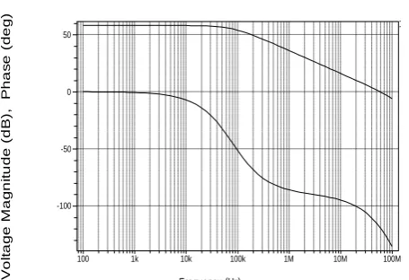
OTA with cacode current source

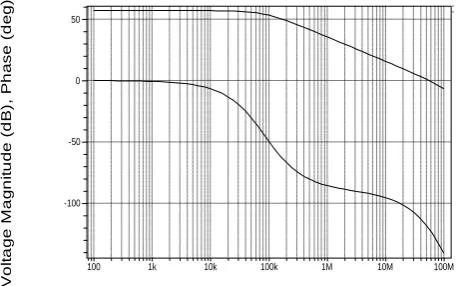
As shown in fig. 14, we present the simulated output frequency response. Where the bode diagram gives a phase margin 62°, a high open loop gain of 57 dB with a large GBW of 58 MHz and a cut-off frequency fb of 82 KHz.

3.1.2 Summary table

Table 6 summarizes the simulation results of the modified tow stage Miller OTA circuit with cascode current source.

Table 6: Summarizes the simulation results of the modified Two-Stage Miller OTA with cascode current

source

Parameters Value Slew rate (SR) 0.13 V/µs

DC Offset 0.5 mV

Gain 57 dB

Average power consumed 2.27 mW Output-voltage swing -1.4 to 1.2 Supply voltage ±1.5V Settling time (St) 17 ns

4. MODIFIED TOW-STAGE MILLER

OTA WITH DESIGNED CURRENT

SOURCE

4.1 Description

fig. 15, in which bias circuit was actively presented by designed current source. This last is consisted of four PMOS transistors (M9A, M10A, M11A, M12A) which formed cascode mirror with weak supply voltage [20].

In this case cascode current mirror can be used for the duplication of current to provide higher output resistance and lower symmetric error. Then the input NMOS transistor (M14A) is based on input voltage (Vin) which is 0 V to obtain low power voltage consumption. On the other hand, after the current goes through PMOS cascode current mirrors, the output obtained is a current value (Iout) by the transistor (M13A), as shown in fig. 16.

A B C D E F G H I J

1 1

2 2

3 3

4 4

5 5

6 6

Rev: 34 13-Dec-2011 11:48 Created: 10-Nov-2011 M8

M5 M6

M1

M2

M4 M7

M3

Cc Cl Vdd

+1.5 V

Vss -1.5 V M9A

M10A

M12A

M11A

M13A M14A Vin

0V _Iout

[image:8.595.316.546.542.714.2]

(9)

A

B

C

D

E

F

G

H

I

J

1 1

2 2

3 3

4 4

5 5

6 6

File: C :\U s ers \radw ene\D es k top\es s ai_TOP_SPIC E\C ON VER TISS__V__I.s c h

M10A

M14A

V dd +1.5 M9A

M11A M12A

M13A V ss -1.5 V in

0V Iout

[image:9.595.60.213.72.233.2]

Fig. 16 : Proposed current source

[image:9.595.310.539.76.219.2]

Table 7 presents the parameters values of op-amp Miller OTA with designed current source.

Table 7: Summarizes the simulation results of the Two-Stage Miller OTA with designed current source

Devices Value

M6 W=220µm L=1µm

M7 W=128µm L=1µm

M9A, M10A W=4µm L=0.35µm M11A, M12A, M13A, M14A W=1µm L=0.35µm Supply voltage Vdd=1.5V Vss= -1.5V

Compensation capacitance Cc = 1.1 pF

4.1.1 Simulations results

The DC analysis of our designed current source is presented in fig. 17, in which the value of current is equal to 28 µA for different values of voltage. In this can we choose input voltage as 0 V to obtain low power consumption.

For low power we

choose : Vin = 0 V

Fig. 17 : DC analysis showing Iout VS input voltage Vin of the

designed current source

100 1k 10k 100k 1M 10M 100M

Frequency (Hz)

-100 -50 0 50

V

o

lt

a

ge

M

a

gn

it

u

de

(

d

B

),

P

h

ase

(d

eg

)

Fig. 18 : Simulated transfer function of amplifier Magnitude (dB) and phase (degree) with the designed current source

As shown in fig. 18, we present the simulated output frequency response. Where the bode diagram gives a phase margin 60°, and a high open loop gain of 57 dB with a large GBW of 55 MHz .

4.1.2 Summary table

[image:9.595.55.297.327.482.2]

Table 8 summarizes the simulation results of the of the Basic Two-Stage Miller OTA

Table 8: Summarizes the simulation results of the of the Basic Two-Stage Miller OTA with designed current source

Parameters Value

Slew rate (SR) 0.1 V/µs

DC Offset 0.5 mV

Gain 57 dB

Average power consumed 1.66 mW Output-voltage swing -1.3 to 1,3 Supply voltage ±1.5V Settling time (St) 15.6 ns

5. COMPARATIVE ANALYSIS

[image:9.595.317.539.390.557.2] [image:9.595.45.302.588.733.2]

(10)

[image:10.595.49.306.106.476.2]

Table 9: Comparison between differents types of Two-stage OTA with technology 0.35µm

6. CONCLUSION

Design of OTA is vital importance in integrated discret-time filters used for design Sigma-Delta converter.

This work presents a novel design method of two-stage CMOS OTA which has been designed and compared with a basic two-stage CMOS OTA. Behavioural simulation indicated that phase margin is 60° to ensure a good stability, gain of 57 dB for ±1.5V without using a gain boosting technique, and GBW of 55 MHz is sufficient to design the ADC converter. The applied technique leads to a significant preservation in gain bandwidth product (GBW), gain (Av), slew rate (SR), and decrease power consumption. The design technique proposed in this paper combines better performance with simplicity of design and suitability for high frequency operation with few modifications on conventional two-stage CMOS OTA and at low power consumption.

These parameters are very important for high frequency, fast settling applications especially in integrated discrete-time filters used for design Sigma-Delta ADC converter.

7. REFERENCES

[1] Chun-Hsien Wu and Yeh-Ching Chung :"Heterogeneous Wireless Sensor Network Deployment and Topology Control Based on Irregular Sensor Model," Advances in Grid and Pervasive Computing Lecture Notes in Computer Science, Volume 4459/2007,2007.

[2] E.J, Duarte-Melo and Mingyan Liu : "Analysis of energy consumption and lifetime of heterogeneous wireless sensor networks," Global Telecommunications Conference , 2002. GLOBECOM ’02. IEEE, vol.1, no., 17-21 Nov 2002.

[3] Vivek Katiyar, Narottam Chand, Surender Soni : "A Survey on Clustering Algorithms for Heterogeneous Wireless Sensor Networks" Int. J. Advanced Networking and Applications Volume: 02, Issue: 04, Pages: 745-754 ,2011

[4] I. F. Akyildiz, W. Su, Y. Sankarasubramaniam, and E. Cayirci : "Wireless sensor networks" A survey Computer Networks, 38(4):393.422, 2002.

[5] T. Bokareva, W. Hu, S. Kanhere, B. Ristic, N. Gordon, T. Bessell, M. Rutten and S. Jha : "Wireless Sensor Networks for Battlefield Surveillance" In roceedings of The Land Warfare Conference (LWC) October 24 – 27, 2006, Brisbane, Australia

[6] YiWu et al, « Multi-Bit Sigma Delta ADC with Reduced Feedback level, Extended Dynamic Range and Increased Tolerance for Analog Imperfections » IEEE 2007 Custom Integrated Circuits Conference (CICC).

[7] Trabelsi.H, Bouzid.Gh, Jaballi.Y, Bouzid.L, Derbel.F and Masmoudi.M : "A 863-870-MHz Spread-Spectrum Direct Conversion Receiver Design for Wireless sensor" IEEE DTIS'06, Tunisia, September, 2006

[8] Ichiro Fujimori, Lorenzo Longo, Armond Hairapetian, Kazushi Seiyama, Steve Kosic, jun Cao and Shu-Lap Chan, “ A 90-dB SNR 2.5-MHz Output-Rate ADC Using Cascaded Multibit Delta-Sigma Modulation at 8X Oversampling Ratio”, IEEE Journal of Solid-State Circuits, vol.35, No 12, December 2000

[9] P. E. Allen and D. R. Holberg, CMOS Analog Circuit Design, 2nd edition, Oxford University Press, 2002 [10] Mezyad M.Amourach and R. L. Geiger : "Gain and

Bandwidth Boosting Techniques for High- Speed Operational Amplifiers, Proceeding" IEEE International Symposium On Circuits and Systems, Sydney, May 2001, pp.232-235

[11] David Johns and Kenneth W. Martin : "Analog Integrated Circuit Design" John Wiley & Sons, 1997. [12] R.J. Baker, H.W. Li, D.E. Boyce, CMOS Circuit Design

Layout and Simulation,Chapter 29, IEEE Press, 1998. [13] Faouzi Chaahoub : "Etude des methodes de conception et

des outils de CAO pour la synthèse des cicuits integrés analogique" thèse doctorat à l’institut national polytechnique de grenoble 1999

[14] Dr. Yannick HERVE : Cours d'Electronique Numérique et de méthodologie de CAO Electronique Conception des système complexes. -mise à jour le 01/03/2010 -wwwensps.u-strasbg.fr/coursen/.../TPE/ampopOTA.ppt Parameter

s

Two-stage Miller

OTA [19]

Modified Two-stage OTA with

cascode current source (Fig. 12)

Two-stage Miller OTA

(Fig. 5)

Modified Two-stage OTA with designed current source

(Fig. 15) Technolog

y

TSMC 0.35µm

AMS 0.35µm

Av gain 48 dB 57 dB 57 dB 57 dB

Average Power consumed

3.4 mW 2.2 mW 3.5 mW 1.66 mW

Phase margin

61° 62° 68° 60°

Slew rate 26 (V/µs) 0.13 (V/µs) 0.2 (V/µs)

0.1 (V/µs) GBW 10 MHz 58 MHz 59 MHz 55 MHz Cut-off

frequency

167 Khz 82 KHz 90 KHz 85 KHz Supply

voltage

3.3 V ±1.5 V ±1.5 V ±1.5 V

Applicatio n

Sigma-Delta modulator of

Digital-Audio

Sigma-Delta Converter

of wireless

sensor receiver

Sigma-Delta Converter

of wireless

sensor receiver

Sigma-Delta Converter of wireless

(11)

[15]F.Silveira, D. Flandre and PGA Jespers : " A gm/ID based methodology for the design of CMOS analog circuits and its application to the synthesis of a silicon-on-insulator micropower OTA" IEEE Journal of solid-state circuits, vol.31, N°. 9, SEPTEMBER 1996

[16]M. Ghovanloo and K. Najafi, “A compact large voltage compliance high output impedance programmable current source for implantable microstimulators,” IEEE Tran. Biomed. Eng., vol. 52, pp. 97-105, Jan.2005. [17]K. E. Jones and R. A. Normann, “An advanced

demultiplexing system for physiological stimulation,” IEEE Trans. Biomed. Eng., vol. 44, no.12, pp. 1210– 1220, Dec. 1997.

[18]S. Boyer, M. Sawan, M. Abdel-Gawad, S. Robin, and M. M. Alhilali, “Implantable selective stimulator to improve

bladder voiding: Design and chronic experiment in dogs,” IEEE Trans. Rehab. Eng., vol. 8, no. 4, pp. 789– 797, Dec. 2000.

[19] Mr. Bhavesh H. Soni, Ms. Rasika N. Dhavse : “Design of Operational Transconductance Amplifier Using 0.35μm Technology,” International Journal of Wisdom Based Computing, Vol. 1 (2), August 2011.

[20] Radwene LAAJIMI, B.HAMDI, N.AYARI: “A Low power Bulk-driven MDAC Synapse,” 2011 International Conference on Applied Electronics (AE)

[21] Medeiro F., del Rio R., de la Rosa J.M., Pérez-Verdù B., A Sigma-Delta modulator design exemple : from specs to

measurements, Baecelonea, May 6-10, 2002 .