Munich Personal RePEc Archive
A dynamic factor model of the coincident
indicators for the US transportation
sector
Lahiri, Kajal and Yao, Wenxiong
Department of Economics, University at Albany-SUNY, Albany, NY
12222, USA
August 2004
Online at
https://mpra.ub.uni-muenchen.de/22360/
A Dynamic Factor Model of the Coincident Indicators
for the U.S. Transportation Sector
Kajal Lahiri
*and Wenxiong Yao
Department of Economics
University at Albany-SUNY
Albany, NY 12222
U.S.A
Running title: Transportation Coincident Index
Abstract
This paper studies the business cycle features of the transportation sector using dynamic
factor models. The transportation reference cycles peak ahead of the economic cycles, but
lag by a few months at troughs. The asymmetric relationship between these two suggests
the usefulness of transportation in monitoring business cycles.
*
1.
INTRODUCTION
Transportation, being an important service-providing sector, represents a significant part
of the U.S. economy. More importantly, transportation plays a vital role in facilitating
economic activity between sectors and across regions. Ghosh and Wolf (1997), in
examining the importance of geographical and sectoral shocks in the U.S. business cycles,
find that transport is one of sectors highly correlated with intra-state and intra-sector
shocks, and is thus crucial in the propagation of business cycles. Interestingly, a number
of transportation indicators were included as part of the twenty-one cyclical indicators in
the original NBER lists by Mitchell and Burns (1938) and Moore (1961, pp. 184-261).
Further efforts to study the role of transportation in monitoring modern business cycles
were hindered largely due to the discontinuation of many transportation indicators such
as freight carloadings in the 1950s and the 1960s. For more information on the history of
cyclical indicators, see the NBER Macrohistory database available online (Feenberg and
Miron, 1997).
Lahiri and Yao (2004) have explored the macroeconomic forecasting potential of a
monthly experimental index measuring the aggregate output of the transportation sector
developed in Lahiri et al. (2003). This transportation services index (TSI), now being
produced by U.S. Department of Transportation, utilizes eight series on freight and
passenger movements from airlines, rail, waterborne, trucking, transit and pipelines
(NAICS codes 481-486) covering around 90% of total for-hire transportation during
1980-2000. TSI is a chained Fisher-ideal index, and is methodologically similar to the
Industrial Production (IP) index, which is one of the four coincident indicators for the
aggregate economy.1 Following the conventional economic indicator analysis (Zarnowitz,
1992), we can use TSI together with other coincident indicators from transportation to
study the business cycles characteristics of this sector, and its relationship to the
aggregate economy. This paper applies dynamic factor models with regime switching
1
(Kim and Nelson, 1998) and without regime switching (Stock and Watson, 1991) to
estimate the composite coincident index (CCI) for the transportation sector.
2.
THE MODEL AND ESTIMATES
Given a set of coincident indicators Yit, their growth rates can be explained by an
unobserved common factor ∆Ct, interpreted as growth in CCI, and some idiosyncratic
dynamics.This defines the measurement equation for each component:
∆Yit = γi∆Ct + eit , (1)
where ∆Yitis logged first difference in Yit.In the state-space representation, ∆Ct itself is to
be estimated. In the transition equations, both the index ∆Ct and eit are processes with AR
representations driven by noise terms wt and εit respectively:
Ф(L) (∆Ct - µst - δ) = wt, (2)
Ψ(L) eit = εit. (3)
These two noise terms are assumed to be independent of each other. The transitions of
different regimes (µst), incorporated in (2), are governed by a Markov process:
µst = µ0 + µ1 St, St = {0, 1}, µ1 > 0, (4)
Prob (St = 1 | St-1 = 1) = p, Prob (St = 0 | St-1 = 0) = q. (5)
Equations (1) ~ (3) define the dynamic factor model while (4) ~ (5) add a nonlinear
regime switching feature to it. Following the NBER tradition and Layton and Moore
(1989), we use four conventional coincident indicators to define the current state of U.S.
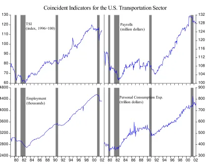
transportation sector. They are: TSI (Y1t) as defined earlier, real aggregate payrolls of
transportation workers (Y2t), real personal consumption expenditure on transportation
services (Y3t), and total employment (Y4t) in this sector. These indicators, plotted in
Figure 1, reflect information on output, income, sales, and labor usage in the
transportation sector.
For the sake of comparison, we first constructed a coincident index for the
transportation sector using the model-free NBER approach, see Conference Board
(2001).2 Using the index of concordance proposed by Harding and Pagan (2002), we
2
This nonparametric approach includes four steps: 1) month-to-month changes (xt) are computed for each
component (Xt) using the conventional formula; 2) the month-to-month changes are adjusted to equalize the
found that the specific cycles of each series are highly synchronized (all values were in
excess of 0.60) with the transportation reference cycle based on the NBER index. To
implement the Kim-Nelson model, we used priors from the estimated Stock-Watson
model. Priors for regime switching parameters were obtained from information provided
by the NBER index. Both models were estimated using computer routines described in
Kim and Nelson (1998). Unlike the Stock-Watson (1989) model specification for the
aggregate economy, personal consumption expenditure and employment in transportation
appear to be somewhat lagging to the current state of transportation.
The final specification and parameter estimates from Stock-Watson and
Kim-Nelson models are reported in Table 1. The two sets of estimates are close except that the
sum of the AR coefficients for the state variable in the Stock-Watson model is
significantly higher, implying more state dependence in the resulting index. This
difference is complemented by a much larger role that employment plays in the
Kim-Nelson model. The latter model also distinguishes between two clear-cut regimes of
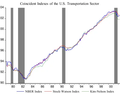
positive and negative growth rates. The estimated transportation CCIs from these two
models are plotted against the NBER index in Figure 2. Compared to the Kim-Nelson
index, the Stock-Watson index agrees more closely with the NBER index throughout the
period. Despite differences in their model formulations and in minor details, their cyclical
movements appear to be very similar to one another and synchronized well with the
NBER-defined recessions for the economy (the shaded areas).
3.
RELATION WITH BUSINESS CYCLES
NBER dating algorithm described in Bry and Boschan (1971) is employed to identify the
turning points for four coincident indicators and the NBER index. The NBER procedure
to define recessions for U.S. economy involves visually identifying clusters of turning
points of all series and minimizing the distance between the turning points in each cluster
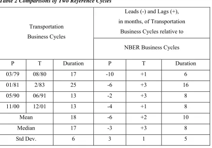
(Layton and Moore, 1989). Following these standard steps, we define the chronology of
cycles in the U.S. transportation sector since January 1979 that includes four major
recessions: 1979:03 ~ 1980:08, 1981:01 ~ 1983:02, 1990:05 ~ 1991:06, and 2000:11 ~
2001:12. These periods are compared against the NBER-defined recessions of the
aggregate economy in Table 2. Overall, there is a one-to-one correspondence between
cycles of the transportation sector and those of the overall economy. However, the
relationship between transportation and the economy is asymmetric at peaks and
troughs.3 Specifically, the transportation sector peaked ahead of the economy by almost 6
months on the average, while at troughs it lagged by two months. In other words,
recessions in the transportation sector lasted longer that the economy-wide recessions by
almost 8 months. Thus, the cycles of this sector can potentially be used to confirm the
NBER dating of U.S. recessions.
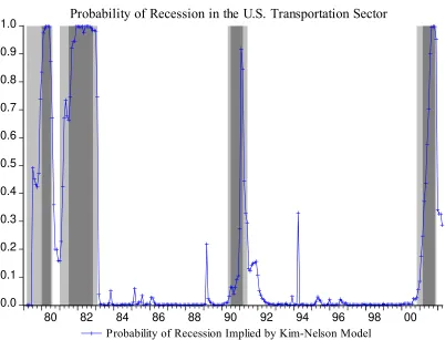
The above analysis is based on the nonparametric procedure practiced by the
NBER Dating Committee. Alternatively, reference cycles can be defined from the
probability of recessions implied by the regime-switching model of Kim and Nelson
(1998). Figure 3 depicts the posterior probability that transportation sector is in a
recession as inferred from the Kim-Nelson model estimation. The darker shaded areas
represent the NBER-defined recessions for the U.S. economy, while the lightly shaded
areas represent recessions in the U.S. transportation sector as defined in Table 2. If we
define the transportation recessions parametrically by taking the first month that the
probability begins to rise (drop) as the trough (peak), the resultant chronology would be
very similar to shaded areas representing transportation recessions defined earlier. The
probabilities in Figure 3 show that, corresponding to each of the four economy-wide
recessions defined by NBER, there is a recession in the transportation sector. The
Kim-Nelson recession probabilities also indicate that the transportation recessions are
consistently longer in duration than the economy-wide recessions. Figure 3 suggests that
the latest recession in the U.S. transportation sector ended in December 2001, which is
just one month after the recently announced NBER trough of the economic recession that
began in March 2001. Interestingly, the finding on the longer duration of transportation
recessions is very similar to that in Moore (1961, pp. 48-51), who used only railway
freight data for his conclusion.
3
4.
CONCLUDING REMARKS
This paper reports certain business cycle features of the U.S. transportation sector using
economic indicator analysis. Four coincident indicators are selected to measure labor
inputs, production, income and spending in this sector. Then composite indexes of these
coincident indicators are created using both the NBER non-parametric method and
dynamic factor models. The resulting indexes are seen to be very similar. We find a close
correspondence between the recessions in the transportation sector and those in the
aggregate economy. However, duration of the transportation recessions is longer than that
of economy-wide recessions by almost 8 months. Further research is needed to explain
the asymmetric lead/lag relationship between the two reference cycles at peaks and
troughs.
ACKNOWLEDGEMENTS
This study has been supported by grants from the Bureau of Transportation Statistics, U.S.
Department of Transportation during 2001-2003. However, the contents of this paper
reflect the views of the authors, who are responsible for the facts and the accuracy of the
information presented herein.
REFERENCES
Bosworth, B. (2001) Output and Productivity in the Transportation Sector: An Overview,
paper presented at ‘Workshop on Transportation Output and Productivity,’ The
Brookings Institution.
Bry, G. and Boschan, C. (1971) Cyclical Analysis of Time Series: Selected Procedures
and Computer Programs, NBER Technical Paper20.
Conference Board (2001) Calculating the Composite Indexes, www.conference-board.org,
revised 01/01.
Feenberg, D. and Miron, J. (1997) Improving the Accessibility of the NBER’s Historical
Data, Journal of Business and Economic Statistics, Vol. 15(3), July, 293-299.
Ghosh, A.R. and Wolf, H.C. (1997) Geographical and Sectoral Shocks in the U.S.
Gordon, R.J. (1992) Productivity in the Transportation Sector, in Griliches, Z. (ed.),
Output Measurement in the Service Sectors, Chicago: University of Chicago Press,
371-428.
Hamilton, J.D. (1989) A New Approach to the Economic Analysis of Nonstationary
Time Series and the Business Cycle, Econometrica, Vol. 57, 357-384.
Harding, D. and Pagan, A. (2002) Dissecting the Cycle: a Methodological Investigation,
Journal of Monetary Economics, Vol. 49, 365-381.
Humphreys, B.R, Maccini, L.J., and Schuh, S. (2001) Input and Output Inventories,
Journal of Monetary Economics, Vol. 47, 347-374.
Kim, C.J. and Nelson, C.R. (1998) Business Cycle Turning Points, A New Coincident
Index, and Tests of Duration Dependence Based on A Dynamic Factor Model with
Regime Switching, The Review of Economics and Statistics, Vol. 80(2), 188-201.
Lahiri, K., Stekler, H.O., Yao, W. and Young, P. (2003) Monthly Output Index for the
US Transportation Sector, Journal of Transportation and Statistics, Vol. 6(2/3), 1-37.
Lahiri, K. and Yao W. (2004) The Predictive Power of an Experimental Transportation
Output Index. Applied Economics Letters, Vol. 11(3), 149-152.
Layton, A. and Moore, G.H. (1989) Leading Indicators for the Service Sector, Journal of
Business and Economic Statistics, Vol. 7(3), 379-386.
Mitchell, W.C. and Burns, A.F. (1938) Statistical Indicators of Cyclical Revivals,
reprinted in Moore, G.H. (ed.) Business Cycle Indicators, Volume I. Princeton, New
Jersey: Princeton University Press for NBER, 1961, 162-183.
Moore, G.H. (1961) Business Cycle Indicators, Volume I. Princeton, New Jersey:
Princeton University Press for NBER.
Stock, J.H. and Waston, M.W. (1991) A Probability Model of the Coincident Economic
Indicators, in Lahiri, K. and Moore, G.H. (eds), Leading Economic Indicators: New
Approaches and Forecasting Records, (Cambridge University Press, Cambridge),
63-89.
Zarnowitz, V. (1992) Business Cycles: Theory, History, Indicators, and Forecasting, The
Figure 1 60 70 80 90 100 110 120 130 100 104 108 112 116 120 124 128 132 2400 2800 3200 3600 4000 4400 4800
80 82 84 86 88 90 92 94 96 98 00 02
300 400 500 600 700 800 900
80 82 84 86 88 90 92 94 96 98 00 02
Coincident Indicators for the U.S. Transportation Sector
TSI (index, 1996=100) Payrolls (million dollars) Employment (thousands)
Personal Consumption Exp. (trillion dollars)
Figure 2
90 92 94 96 98 100 102 104
80 82 84 86 88 90 92 94 96 98 00
NBER Index Stock-Watson Index Kim-Nelson Index
Coincident Indexes of the U.S. Transportation Sector
Figure 3
0.0 0.1 0.2 0.3 0.4 0.5 0.6 0.7 0.8 0.9 1.0
80 82 84 86 88 90 92 94 96 98 00
Probability of Recession Implied by Kim-Nelson Model
Probability of Recession in the U.S. Transportation Sector
* Darker shaded areas represent NBER-defined recessions for the U.S. economy; lightly shaded
Table 1 Estimates of the Transportation Coincident Index Models
Kim-Nelson Model Stock-Watson Model
Posterior Variables Parameters
Estimate s.e. Prior
Mean s.e. Median
∆Ct Φ1 0.775 0.167 0.775 0.127 0.119 0.114
(State Variable) Φ 2 0.107 0.162 0.107 0.121 0.085 0.124
∆Y1t γ1 0.171 0.057 0.1 0.136 0.028 0.136
(Output) φ11 -0.519 0.067 -0.2 -0.637 0.057 -0.638
φ 12 -0.067 0.017 0 -0.401 0.057 -0.401
σ12
5.181 0.480 2 0.652 0.057 0.648
∆Y2t γ2 0.148 0.048 0.1 0.173 0.042 0.172
(Payrolls) φ 21 -0.162 0.077 -0.1 -0.216 0.061 -0.216
σ22
2.107 0.210 2 0.782 0.071 0.778
∆Y3t γ3 1.485 0.631 1.5 0.059 0.060 0.059
(Personal γ31 -1.364 0.626 -1.4 -0.041 0.059 -0.039
Consumption φ 31 -0.149 0.122 -0.1 -0.388 0.060 -0.388
Exp.) σ32 2.443 1.831 2 0.849 0.076 0.844
∆Y4t γ4 0.110 0.021 0.1 0.548 0.081 0.557
(Employment) φ 41 -0.006 0.357 -0.1 -0.025 0.084 -0.026
σ42
0.072 0.015 2 0.125 0.081 0.120
P00 0.967 0.926 0.066 0.945
P11 0.986 0.985 0.012 0.988
µ0 -0.869 -1.822 0.554 -1.727
µ1 0.745 2.208 0.580 2.110
δ - 0.356 0.038 0.359
Table 2 Comparisons of Two Reference Cycles
Leads (-) and Lags (+),
in months, of Transportation
Business Cycles relative to Transportation
Business Cycles
NBER Business Cycles
P T Duration P T Duration
03/79 08/80 17 -10 +1 6
01/81 2/83 25 -6 +3 16
05/90 06/91 13 -2 +3 8
11/00 12/01 13 -4 +1 8
Mean 18 -6 +2 10
Median 17 -3 +3 8