R E S E A R C H
Open Access
Simultaneous and semi-alternating
projection algorithms for solving split
equality problems
Qiao-Li Dong
*and Dan Jiang
*Correspondence:
Tianjin Key Laboratory for Advanced Signal Processing, College of Science, Civil Aviation University of China, Tianjin, 300300, China
Abstract
In this article, we first introduce two simultaneous projection algorithms for solving the split equality problem by using a new choice of the stepsize, and then propose two semi-alternating projection algorithms. The weak convergence of the proposed algorithms is analyzed under standard conditions. As applications, we extend the results to solve the split feasibility problem. Finally, a numerical example is presented to illustrate the efficiency and advantage of the proposed algorithms.
MSC: 90C47; 49J35
Keywords: simultaneous projection algorithm; semi-alternating projection algorithm; maximal monotone operator; split equality problem
1 Introduction
LetH1,H2andH3be real Hilbert spaces, letC⊆H1andQ⊆H2be two nonempty closed
convex sets, and letA:H1→H3andB:H2→H3be two bounded linear operators. In this article, we consider the classical split equality problem (SEP), which was first introduced by Moudafi [1]. The SEP can mathematically be formulated as follows:
Find x∈C,y∈Q such that Ax=By. (1)
Throughout this paper, assume that SEP (1) is consistent and denote by
={x∈C,y∈Q:Ax=By}
the solution of SEP (1). Thenis closed, convex and nonempty.
The split equality problem (1) is actually an optimization problem with weak coupling in the constraint (see [1] for details) and its interest covers many situations, for instance, in domain decomposition for PDEs, game theory and intensity-modulated radiation ther-apy (IMRT). In domain decomposition for PDEs, this equals to the variational form of a PDE in a domain that can be decomposed into two non-overlapping subdomains with a common interface (see, e.g., [2]). In decision sciences, this allows to consider agents who interplay only via some components of their decision variables (see, e.g., [3]). In IMRT,
this amounts to envisaging a weak coupling between the vector of doses absorbed in all voxels and that of the radiation intensity (see [4] for further details). Attouch [5] pointed out more applications of the SEP in optimal control theory, surface energy and potential games, whose variational form can be seen as a SEP.
Next we present an example, in which a separable optimization problem can be rewrit-ten as a split equality problem.
Example 1.1 Consider the separable optimization problem
minimizef(x) +g(y)
subject toAx=By,
(2)
withx∈RN andy∈RM, whereA∈RJ×N andB∈RJ×M. Assume thatf andgare convex
and the solution set of problem (2) is nonempty.
Set C=argmin{f(x)|x∈RN} andQ=argmin{g(y)|y∈RM}. Then the optimization
problem (2) equals to the following split equality problem:
Find x∈C,y∈Q such that Ax=By. (3)
A great deal of literature on algorithms for solving SEP has been published, most of which are projection methods [1–3, 6–11]. Based on the classical projection gradient al-gorithm, Byrne and Moudafi [12] introduced the following alal-gorithm, which is also called the simultaneous iterative method [13]:
⎧ ⎨ ⎩
xk+1=P
C(xk–βkA∗(Axk–Byk)), yk+1=PQ(yk+βkB∗(Axk–Byk)),
(4)
whereβk∈(ε, 2/(λA+λB) –ε),λAandλBare the operator (matrix) normsAandB(or
the largest eigenvalues ofA∗AandB∗B), respectively. To determine stepsizeβk, one needs
first to calculate (or estimate) the operator normsAandB. In general, it is difficult or
even impossible. On the other hand, even if we know the norm ofAandB, the algorithm (4) method with fixed stepsize may be slow.
In order to deal with this, the authors [9] introduced a self-adaptive projection algo-rithm, in which the stepsize is computed by using an Armijo search.
Define the functionF:H1×H2→H1by
F(x,y) =A∗(Ax–By),
and the functionG:H1×H2→H2by
G(x,y) =B∗(By–Ax).
Algorithm 1.1 Given constantsσ0> 0,α∈(0, 1),θ∈(0, 1) andρ∈(0, 1). Letx0∈H1and y0∈H2be taken arbitrarily. Fork= 0, 1, 2, . . . , compute
⎧ ⎨ ⎩
uk=P
C(xk–βkF(xk,yk)),
vk=PQ(yk–βkG(xk,yk)), (5)
whereβkis chosen to be the largestβ∈ {σk,σkα,σkα2, . . .}satisfying
β2Fxk,yk–Fuk,vk2+Gxk,yk–Guk,vk2
≤θ2xk–uk2+yk–vk2. (6)
Compute
⎧ ⎨ ⎩
xk+1=PC(xk–βkF(uk,vk)),
yk+1=PQ(yk–βkG(uk,vk)). (7)
If
βk2Fxk,yk–Fxk+1,yk+12+Gxk,yk–Gxk+1,yk+12
≤ρ2xk–xk+12+yk–yk+12, (8)
then setσk=σ0; otherwise, setσk=βk.
In fact, Algorithm 1.1 can be seen as an extension of the classical extragradient method first proposed by Korpelevich [14]. Notice that, in Algorithm 1.1, the stepsize of the pre-diction (5) and that of the correction (7) are equal. Thus these two steps seem to be ‘sym-metric’.
Recently, Chuang and Du [15] proposed the following projection algorithm (which is called the hybrid projected Landweber algorithm).
Algorithm 1.2 Given constantsσ> 0,α∈(0, 1) andθ∈(0, 1), letx0∈H
1andy0∈H2be
taken arbitrarily. Fork= 0, 1, 2, . . . , compute
⎧ ⎨ ⎩
uk=PC(xk–βkF(xk,yk)), vk=P
Q(yk–βkG(xk,yk)),
whereβkis chosen via (6) and (8). Compute next iteratesxk+1andyk+1by ⎧
⎨ ⎩
xk+1=P
C(xk–ρkck),
yk+1=PQ(yk–ρkdk), (9)
where
⎧ ⎨ ⎩
and
ρk:=
xk–uk,c
k +yk–vk,dk
ck2+dk2 . (10)
Note that Algorithm 1.2 withρk≡1 in (9) can be seen as a special case of Tseng’s method
[8, 16]. The projections in the second step of Tseng’s method are made onto two nonempty closed convex setsX⊆H1andY⊆H2, other thanCandQ.XandYcan be any sets such that the intersections ofXandC(andY andQ) are nonempty, and they may be taken to have simple structures so that the projections onto them are easy to calculate.
Chuang and Du [15] proved the convergence of Algorithm 1.2 and also presented the convergence property of Algorithm 1.2 as follows:
xk+1–x∗2+yk+1–y∗2
≤xk–x∗2+yk–y∗2–ρk2ck2+dk2, (11)
where (x∗,y∗)∈.
The stepsizeβkin Algorithms 1.1 and 1.2 is obtained through the Armijo search (6). In
general, the computational cost of a self-adaptive algorithm is large, since one may need to calculate (5) several times to get the stepsizeβk.
To overcome this difficulty, the authors [17] introduced a projection algorithm for which the stepsize does not depend on the operator normsAandB, and one can directly compute the stepsize instead of using the Armijo search.
Algorithm 1.3 Choose initial guessesx0∈H1,y0∈H2arbitrarily. Assume that thekth
iteratexk∈C,yk∈Qhas been constructed andAxk–Byk= 0; then we calculate the (k+ 1)th iterate (xk+1,yk+1) via the formula
⎧ ⎨ ⎩
xk+1=P
C(xk–βkA∗(Axk–Byk)),
yk+1=PQ(yk+βkB∗(Axk–Byk)), (12)
where the stepsizeβkis chosen in such a way that
βk=σkmin
Axk–Byk2
A∗(Axk–Byk)2,
Axk–Byk2
B∗(Axk–Byk)2 , (13)
where 0 <σk< 1. IfAxk–Byk= 0, then (xk+1,yk+1) = (xk,yk) is a solution of SEP (1) and the
iterative process stops; otherwise, we setk:=k+ 1 and go onto (12) to evaluate the next iterate (xk+2,yk+2).
Note that the choice in (13) of the stepsizeβkis independent of the normsAandB.
Algorithm 1.4 Choose initial guessesx0,x1∈H1,y0,y1∈H2arbitrarily. Compute ⎧
⎪ ⎪ ⎨ ⎪ ⎪ ⎩
(x¯k,y¯k) = (xk,yk) +α
k(xk–xk–1,yk–yk–1), xk+1=PC(¯xk–βkA∗(Ax¯k–By¯k)),
yk+1=PQ(¯yk+βkB∗(Ax¯k–By¯k)),
(14)
whereαk∈(0, 1) and the stepsizeγkis chosen in the same way as (13).
They showed the weak convergence of Algorithm 1.4 under some conditions on the inertial parameterαk.
In fact, Algorithm 1.4 can be seen as a FISTA (fast iterative shrinkage-thresholding al-gorithm) introduced by Beck and Teboulle [21] to solve the linear inverse problems, if we
take the inertial parameterαk=ttkk–1+1, wheret1= 1 andtk+1= 1+
1+4tk2
2 ,k≥1, and choose a
constant stepsizeβk or chooseβkvia a backtracking stepsize rule. A shortcoming of the
method of Beck and Teboulle is that they could not prove the convergence of the iterative sequence (xk,yk). Chambolle and Dossal [22] improved the choice of the inertial
param-eter, tookαk=k–1k+a, wherea> 2, and presented the convergence of the iterative sequence
(xk,yk).
In this paper, inspired by the work in [17, 23, 24], we introduce two simultaneous pro-jection algorithms by improving the stepsizesβk andρk of the second step (7) and (9)
in Algorithms 1.1 and 1.2, respectively. We also present two alternating projection algo-rithms, in which we take an alternating technique in the first step.
The structure of the paper is as follows. In the next section, we present some concepts and lemmas which will be used in the main results. In Section 3, two classes of projection algorithms are provided and their weak convergence is analyzed. In Section 4, we extend the results to the split feasibility problem. In the final section, some numerical results are provided, which show the advantages of the proposed algorithms.
2 Preliminaries
LetH be a real Hilbert space with the inner product·,· and the induced norm · , and letDbe a nonempty, closed and convex subset ofH. We writexkxto indicate that the sequence{xk}∞
k=0converges weakly toxandxk→xto indicate that the sequence
{xk}∞
k=0converges strongly tox. Given a sequence{xk}k=0∞ , denote byωw(xk) its weakω
-limit set, that is, any x∈ωw(xk) such that there exists a subsequence{xkj}∞j=0 of{xk}∞k=0
which converges weakly tox.
In this paper, an important tool of our work is the projection. LetH be a real Hilbert space andCbe a closed convex subset ofH. Recall that theprojectionfromHonto
C, denoted byPC, is defined in such a way that, for eachx∈H,PC(x) is the unique point
inCsuch that
x–PC(x)=min
x–z:z∈C.
The following two lemmas are useful characterizations of projections.
Lemma 2.1([25]) Given x∈H and z∈C.Then z=PC(x)if and only if
Lemma 2.2([25, 26]) For any x,y∈H and z∈C,it holds (i) PC(x) –PC(y) ≤ x–y;
(ii) PC(x) –z2≤ x–z2–PC(x) –x2.
Definition 2.1 Thenormal coneofCatv∈C, denoted byNC(v), is defined as
NC(v) :=d∈H| d,y–v ≤0 for ally∈C.
Definition 2.2 LetA:H⇒2Hbe a point-to-set operator defined on a real Hilbert space
H. The operatorAis called amaximal monotone operatorifAismonotone, i.e.,
u–v,x–y ≥0 for allu∈A(x) andv∈A(y),
and the graphG(A) ofA,
G(A) :=(x,u)∈H×H|u∈A(x),
is not properly contained in the graph of any other monotone operator.
It is clear [27, Theorem 3] that a monotone mappingAis maximal if and only if, for any (x,u)∈H×H, ifu–v,x–y ≥0 for all (v,y)∈G(A), then it follows thatu∈A(x).
Lemma 2.3([26]) Let D be a nonempty,closed and convex subset of a Hilbert space H.Let
(xk)be a bounded sequence which satisfies the following properties: (i) every limit point of{xk}∞
k=0lies inD; (ii) limn→∞xk–xexists for everyx∈D. Then{xk}converges weakly to a point in D.
3 Main results
In this section, we present two classes of projection algorithms and establish their weak convergence under standard conditions.
3.1 Simultaneous projection algorithms
LetS=C×Q∈H:=H1×H2. DefineK= [A, –B] :H1×H2→H1×H2, and letK∗be the adjoint operator ofK, then the original problem (1) can be modified as
Find z= (x,y)∈S such that Kw= 0. (15)
Note that if the solution set of (15) is nonempty, it equals the following minimization problem:
min z∈S
1 2Kz
2, (16)
Inspired by Cai [24] and Dong et al. [17], we propose two new simultaneous projection algorithms by improving the stepsizes in the second step of Algorithms 1.1 and 1.2.
Algorithm 3.1 Given constantsσ> 0,α∈(0, 1),θ∈(0, 1) andρ∈(0, 1), letz0= (x0,y0)∈
H=H1×H2be taken arbitrarily. Fork= 0, 1, 2, . . . , compute
wk=PS
zk–βkK∗K
zk, (17)
whereβkis chosen to be the largestβ∈ {σk,σkα,σkα2, . . .}satisfying
βK∗Kzk–K∗Kwk≤θzk–wk. (18)
Compute next iterateszk+1by
zIk+1=zk–γρkd
zk,wk, (19)
or
zIIk+1=PS
zk–γ βkρkK∗K
wk, (20)
whereγ ∈[0, 2),
dzk,wk:=zk–wk–βk
K∗Kzk–K∗Kwk, (21)
and
ρk:=
zk–wk,d(zk,wk) +β
kK(wk)2
d(zk,wk)2 . (22)
If
βkK∗K
zk–K∗Kzk+1≤ρzk–zk+1, (23)
then setσk=σ0; otherwise, setσk=βk.
Remark 3.1 Letz= (x,y). Then we have (see Section 4.4.1 in [28])
PS(z) = (PCx,PQy).
It is easy to see
K∗Kz=
A∗A –A∗B
–B∗A B∗B x y
=
A∗(Ax–By)
B∗(By–Ax)
.
Define the functionF:H1×H2→H1by
and the functionG:H1×H2→H2by
G(x,y) =B∗(By–Ax). (25)
By settingzk= (xk,yk) andwk= (uk,vk), Algorithm 3.1 can be rewritten as follows: Fork= 0, 1, 2, . . . , compute
⎧ ⎨ ⎩
uk=P
C(xk–βkF(xk,yk)),
vk=PQ(yk–βkG(xk,yk)), (26)
whereβkis chosen to be the largestβ∈ {σk,σkα,σkα2, . . .}satisfying
β2Fxk,yk–Fuk,vk2+Gxk,yk–Guk,vk2
≤θ2xk–uk2+yk–vk2. (27)
Compute next iteratesxk+1andyk+1by ⎧
⎨ ⎩
xk+1
I =xk–γρkck,
yk+1I =yk–γρkdk, (28)
or
⎧ ⎨ ⎩
xk+1II =PC(xk–γ βkρkF(uk,vk)), yk+1II =PQ(yk–γ β
kρkG(uk,vk)),
(29)
whereγ ∈[0, 2),
⎧ ⎨ ⎩
ck:= (xk–uk) –β
k(F(xk,yk) –F(uk,vk)); dk:= (yk–vk) –βk(G(xk,yk) –G(uk,vk)),
(30)
and
ρk:=
xk–uk,ck +yk–vk,dk +βkAuk–Bvk2
ck2+dk2 . (31)
If
βk2Fxk,yk–Fxk+1,yk+12+Gxk,yk–Gxk+1,yk+12
≤ρ2xk–xk+12+yk–yk+12, (32)
then setσk=σ0; otherwise, setσk=βk.
For convenience, we call the projection algorithms which use update forms (19) (or (28)) and (20) (or (29)) Algorithm 3.1(I) and Algorithm 3.1(II), respectively.
(i) The only difference between Algorithm 3.1(II) and Algorithm 1.1 is that they use different stepsizes in the definitions ofxk+1andyk+1.
(ii) There are two differences between Algorithm 3.1(I) and Algorithm 1.2. Firstly, the stepsizeρkin (10) of Algorithm 3.1(I) is larger than that in (36) of Algorithm 1.2. Secondly, there are no projections on the second step (19).
Remark 3.3 By the definitions ofdkin (21), the projection equation (17) can be written as
wk=PS
wk–βkK∗K
wk–dzk,wk.
So, from Lemma 2.1 we have
z–wk,βkK∗K
wk–dzk,wk≥0, ∀z∈S. (33)
Lemma 3.1 The search rule(18)is well defined.Besidesβ≤βk≤σ,where
β=min
σ, αθ
K2 . (34)
Proof Obviously,βk≤σk≤σ0. In the latter case, we know thatβk/αmust violate
inequal-ity (18), that is,
K∗Kzk–K∗Kwk≥θz k–wk βk/α
. (35)
On the other hand, we have
K∗Kzk–K∗Kwk≤ K2zk–wk. (36)
Consequently, we get (34).
Lemma 3.2 Let(zk)and(wk)be generated by Algorithm3.1,and let dkandρkbe given by
(21)and(36),respectively.Then we have
ρk≥
1 –θ
1 +θ2. (37)
Proof By the Cauchy-Schwarz inequality, we have
zk–wk,dzk,wk
=zk–wk2–βk
zk–wk,K∗Kzk–K∗Kwk
≥zk–wk2–βkzk–wkK∗K
zk–K∗Kwk
≥zk–wk2–θzk–wk2
By using zk–wk,K∗K(zk) –K∗K(wk) =K(zk) –K(wk),K(zk) –K(wk) =K(zk) – K(wk)2, we have
dzk,wk2=zk–wk2+βk2K∗Kzk–K∗Kwk2
– 2βk
zk–wk,K∗Kzk–K∗Kwk
≤zk–wk2+θ2zk–wk2– 2βkK
zk–Kwk2
≤1 +θ2zk–wk2.
So, we get (37).
Lemma 3.3 Let(zk)and(wk)be generated by Algorithm3.1,and let d
kbe given by(21). Then,for all(z∗)∈,we have
zk–z∗,dzk,wk≥ρkd
zk,wk2. (39)
Proof Take arbitrarilyz∗∈, that is,z∗∈S, andK(z∗) = 0. By settingz=z∗in (33), we get
z∗–wk,βkK∗Kwk–dzk,wk≥0,
which implies that
wk–z∗,dzk,wk≥βk
wk–z∗,K∗Kwk.
It is easy to show that
wk–z∗,K∗Kwk=Kwk–z∗,Kwk=Kwk2. (40)
So we have
zk–z∗,dzk,wk=zk–wk,dzk,wk+wk–z∗,dzk,wk
≥zk–wk,dzk,wk+βkK
wk2
=ρkd
zk,wk2,
which implies (39).
Theorem 3.1 Let(zk)be generated by Algorithm3.1(I).Ifis nonempty,then we have zk+1
I –z∗ 2
≤zk–z∗2–γ(2 –γ)ρ2 kd
zk,wk2, ∀z∗∈ (41)
and(zk)converges weakly to a solution of SEP(1).
Proof Letz∗∈, that is,z∗∈S, andK(z∗) = 0. Then, from (39), we have
zk+1I –z∗2=zk–z∗2+γ2ρk2dzk,wk2– 2γρk
zk–z∗,dzk,wk
≤zk–z∗2+γ2ρk2dzk,wk2– 2γρk2dzk,wk2
which yields (41). Sinceγ ∈(0, 2), (42) implies that the sequence (zk–z∗2) is decreasing
and thus converges. Moreover, (zk) is bounded. This implies that
lim k→∞ρ
2 kd
zk,wk2= 0. (43)
From the definition ofρk, Lemmas 3.1 and 3.2, we have
ρk2dzk,wk2=ρk
zk–wk,dzk,wk+βkK
wk2
≥ρk
(1 –θ)zk–wk2+βkK
wk2
≥(1 –θ)2 1 +θ2 z
k–wk2+ 1 –θ
1 +θ2βK
wk2,
which implies
zk–wk2≤ 1 +θ 2
(1 –θ)2ρ 2 kd
zk,wk2
and
Kwk2≤ 1 +θ 2
(1 –θ)βρ 2 kd
zk,wk2.
Using (43), we get
lim k→∞z
k–wk= 0 (44)
and
lim k→∞K
wk= 0.
By the boundedness ofK, we get
lim k→∞K
zk= 0. (45)
Letzˆ∈ωw(zk), then there exists a subsequence (zki) of (zk) which converges weakly to
ˆ
z. From (44), it follows that the subsequence (wki) also converges weakly tozˆ. We will
show thatˆzis a solution of SEP (1). The weak convergence of (K(zki)) toK(ˆz) and lower
semicontinuity of the squared norm imply that
K(ˆz)≤lim inf i→∞ K
zki= 0,
that is,K(ˆz) = 0. By noting that the equality in (17) can be rewritten as
zki–wki βki
and that the graph of the maximal monotone operatorNSis weakly-strongly closed, and by passing to the limit in the last inclusions, we obtain, from (44) and (45), that
ˆ
z∈S.
Hencezˆ∈. Now we can apply Lemma 2.3 toD:=to get that the full sequence (zk)
converges weakly to a point in. This completes the proof.
Remark 3.4 By using Remark 3.1, the contraction inequality (41) can be rewritten as fol-lows:
xk+1I –x∗2+yk+1I –y∗2≤xk–x∗2+yk–y∗2–γ(2 –γ)ρk2ck2+dk2
. (46)
It is obvious that theρkin (31) is larger than that in (10). Letγ = 1. Comparing (46) and
(11), we claim that Algorithm 3.1(I) has a better contraction property than Algorithm 1.2.
Theorem 3.2 Let(zk)be generated by Algorithm3.1(II).Assume thatis nonempty.Then we have
zk+1II –z∗2≤zk–z∗2–γ(2 –γ)ρk2dzk,wk2–zIk+1–zk+1II 2, ∀z∗∈. (47)
Furthermore, (zk)converges weakly to a solution of SEP(1).
Proof Letz∗∈, that is,z∗∈S, andK(z∗) = 0. Using Lemma 2.2(ii), we have
zk+1II –z∗2≤zk–γ βkρkK∗K
wk–z∗2–zk–γ βkρkK∗K
wk–zk+1II 2
=zk–z∗2–zk–zk+1II 2– 2γ βkρk
zIIk+1–z∗,K∗Kwk. (48)
By settingz=zk+1II in (33), we get
–2γ βkρk
zIIk+1–wk,K∗Kwk
≤–2γρk
zk+1II –wk,dzk,wk
= –2γρk
zk–wk,dzk,wk– 2γρk
zk+1II –zk,dzk,wk. (49)
It holds
–2γρk
zk+1II –zk,dzk,wk= –zk–zk+1II –γρkdzk,wk2
+zk–zIIk+12+γ2ρk2dzk,wk2. (50)
Substituting (50) in the right-hand side of (49) and usingzk–γρkd(zk,wk) =zk+1
I , we obtain
–2γ βkρk
zIIk+1–wk,K∗Kwk
≤–2γρk
zk–wk,dzk,wk–zk+1I –zk+1II 2
From (40), we get
–2γ βkρk
wk–w∗,K∗Kwk= –2γ βkρkK
wk2. (52)
So, adding (51) and (52) and using the definition ofρk, we obtain
–2γ βkρk
zIIk+1–z∗,K∗Kwk
≤–2γρk
zk–wk,dzk,wk+βkK
wk2
–zk+1I –zIIk+12+zk–zIIk+12+γ2ρ2kdzk,wk2
≤–2γρk2dzk,wk2+γ2ρk2dzk,wk2–zIk+1–zIIk+12+zk–zk+1II 2
≤–γ(2 –γ)ρk2dzk,wk2–zIk+1–zk+1II 2+zk–zk+1II 2. (53)
Adding (48) and (53), we obtain (47). Employing arguments which are similar to those used in the proof of Theorem 3.1, we obtain that the whole sequence (zk) weakly converges to
a solution of SEP (1), which completes proof.
Remark 3.5 Comparing inequalities (41) and (47), we conclude that Algorithm 3.1(II) seems to have a better contraction property than Algorithm 3.1(I) sincezk+1II is closer toz∗
thanzk+1
I whenzkis the same.
3.2 Semi-alternating projection algorithms
Inspired by Algorithm 2.2 in [15] and based on Algorithm 3.1, we present two semi-alternating projection algorithms, whose name comes from an semi-alternating technique taken in the first step.
Algorithm 3.2 Given constantsσ0> 0,α∈(0, 1),θ∈(0, 1) andρ∈(0, 1), letx0∈H1and y0∈H2be taken arbitrarily.
Fork= 0, 1, 2, . . . , compute
⎧ ⎨ ⎩
uk=P
C(xk–βkF(xk,yk)),
vk=PQ(yk–βkG(uk,yk)), (54)
whereβkis chosen to be the largestβ∈ {σk,σkα,σkα2, . . .}satisfying
β2Fxk,yk–Fuk,vk2+Guk,yk–Guk,vk2
≤θ2xk–uk2+yk–vk2. (55)
Compute next iteratesxk+1andyk+1by ⎧
⎨ ⎩
xk+1
I =xk–γρkck,
or
⎧ ⎨ ⎩
xk+1
II =PC(xk–γ βkρkF(uk,vk)), yk+1II =PQ(yk–γ βkρkG(uk,vk)),
(57)
whereγ ∈[0, 2),
⎧ ⎨ ⎩
ck:= (xk–uk) –βk(F(xk,yk) –F(uk,vk)); dk:= (yk–vk) –βk(G(uk,yk) –G(uk,vk)),
(58)
and
ρk:=
xk–uk,ck +yk–vk,dk +β
kAuk–Bvk2
ck2+dk2 . (59)
If
βk2Fxk,yk–Fxk+1,yk+12+Gxk,yk–Gxk+1,yk+12
≤ρ2xk–xk+12+yk–yk+12, (60)
then setσk=σ0; otherwise, setσk=βk.
For convenience, we call the projection algorithms which use update forms (56) and (57) Algorithm 3.2(I) and Algorithm 3.2(II), respectively.
Remark 3.6 By the definitions ofckanddkin (58), the projection equation (54) can be written as
⎧ ⎨ ⎩
uk=P
C(uk– (βkF(uk,vk) –ck)), vk=PQ(vk– (βkG(uk,vk) –dk)).
So, from Lemma 2.1 we have
⎧ ⎨ ⎩
x–uk,β
kF(uk,vk) –ck ≥0, ∀x∈C,
y–vk,βkG(uk,vk) –dk ≥0, ∀y∈Q. (61)
Lemma 3.4 The search rule(55)is well defined.Besidesβ∗≤βk≤σ0,where
β∗=min
σ0, αθ
√ 2A2,
αθ
B2(A2+B2) . (62)
Proof Obviously,βk≤σk≤σ0. In the latter case, we know thatβk/αmust violate
inequal-ity (55), that is,
β2/α2Fxk,yk–Fuk,vk2+Guk,yk–Guk,vk2
On the other hand, we have
Fxk,yk–Fuk,vk2+Guk,yk–Guk,vk2
=A∗Axk–Byk–A∗Auk–Bvk2+B∗Byk–Auk–B∗Bvk–Auk2
≤ A2Axk–Auk+Byk–Bvk2+B4yk–vk2
≤2A2A2xk–uk2+B2yk–vk2+B4yk–vk2
≤2A4xk–uk2+B22A2+B2yk–vk2
≤max2A4+B22A2+B2xk–uk2+yk–vk2.
So, we get (62).
Lemma 3.5 Let(xk,yk)and(uk,vk)be generated by Algorithm3.2 ,and let ck,dkandρ k be given by(58)and(59),respectively.Then we have
ρk≥
1 –θ
1 +θ2.
Proof By the Cauchy-Schwarz inequality, we have
xk–uk,ck
+yk–vk,dk
=xk–uk2+yk–vk2–βk
xk–uk,Fxk,yk–Fuk,vk
–βk
yk–vk,Guk,yk–Guk,vk
≥xk–uk2+yk–vk2
–βkxk–ukF
xk,yk–Fuk,vk+yk–vkGuk,yk–Guk,vk. (63)
It holds
βk2xk–ukFxk,yk–Fuk,vk+yk–vkGuk,yk–Guk,vk2
=βk2xk–uk2Fxk,yk–Fuk,vk2+yk–vk2Guk,yk–Guk,vk2
+ 2xk–ukFxk,yk–Fuk,vkyk–vkGuk,yk–Guk,vk
≤βk2xk–uk2Fxk,yk–Fuk,vk2+yk–vk2Guk,yk–Guk,vk2
+xk–uk2Guk,yk–Guk,vk2+yk–vk2Fxk,yk–Fuk,vk2
=βk2Fxk,yk–Fuk,vk2+Guk,yk–Guk,vk2xk–uk2+yk–vk2
≤θ2xk–uk2+yk–vk22. (64)
So, we obtain
xk–uk,ck+yk–vk,dk
≥xk–uk2+yk–vk2–θxk–uk2+yk–vk2
From the definition ofFandG, we have
ck2+dk2
=xk–uk2+yk–vk2
+βk2Fxk,yk–Fuk,vk2+Guk,yk–Guk,vk2
– 2βk
xk–uk,Fxk,yk–Fuk,vk+yk–vk,Guk,yk–Guk,vk
≤xk–uk2+yk–vk2+θ2xk–uk2+yk–vk2
– 2βk
Axk–uk,Axk–uk–Byk–vk
–Byk–vk,Auk–uk–Byk–vk
≤xk–uk2+yk–vk2+θ2xk–uk2+yk–vk2
– 2βkA
xk–uk2–Axk–uk,Byk–vk+Byk–vk2. (66)
Since
–2βkA
xk–uk2–Axk–uk,Byk–vk+Byk–vk2
≤–2βkA
xk–uk2–Axk–ukByk–vk+Byk–vk2
≤–2βk
Axk–uk2–1
2A
xk–uk2+Byk–vk2+Byk–vk2
≤–βkA
xk–uk2+Byk–vk2,
by (66), we get
ck2+dk2
≤1 +θ2xk–uk2+yk–vk2–βkA
xk–uk2+Byk–vk2
≤1 +θ2xk–uk2+yk–vk2. (67)
Combining (65) and (67), we complete the proof.
Lemma 3.6 Let(xk,yk)and(uk,vk)be generated by Algorithm3.2,and let c
kand dk be given by(58).Then,for all(x∗,y∗)∈,we have
xk–x∗,ck+yk–y∗,dk≥ρk
ck2+dk2.
Proof Take arbitrarily (x∗,y∗)∈, that is,x∗∈C,y∗∈Q, andAx∗=By∗. By setting (x,y) = (x∗,y∗) in (61), we get
⎧ ⎨ ⎩
x∗–uk,β
kF(uk,vk) –ck ≥0,
which implies that
⎧ ⎨ ⎩
uk–x∗,ck ≥β
kuk–x∗,F(uk,vk) ,
vk–y∗,d
k ≥βkvk–y∗,G(uk,vk).
By the definition ofFandG, we have
uk–x∗,Fuk,vk+vk–y∗,Guk,vk
=uk–x∗,A∗Auk–Bvk+vk–y∗,B∗Bvk–Auk
=Auk–Ax∗,Auk–Bvk+Bvk–By∗,Bvk–Auk
=Auk–Bvk–Ax∗–By∗,Auk–Bvk
=Auk–Bvk2, (68)
and
xk–x∗,ck+yk–y∗,dk
=xk–uk,ck+yk–vk,dk+uk–x∗,ck+vk–y∗,dk
≥xk–uk,ck+yk–vk,dk+βkAuk–Bvk2
=ρk
ck2+dk2.
So, we complete the proof.
Theorem 3.3 Let(xk,yk)be generated by Algorithm3.2(I).Ifis nonempty,then we have xk+1I –x∗2+yk+1I –y∗2
≤xk–x∗2+yk–y∗2– (2 –γ)γρk2ck2+dk2, ∀x∗,y∗∈, (69)
and(xk,yk)converges weakly to a solution of SEP(1).
Proof Let (x∗,y∗)∈, that is,x∗∈C,y∗∈Q, andAx∗=By∗. Then we have
xk+1I –x∗2=xk–γρkck–x∗2
=xk–x∗2+γ2ρk2ck2– 2γρk
xk–x∗,ck.
Similarly, we get
yk+1I –y∗2=yk–y∗2+γ2ρk2dk2– 2γρk
yk–y∗,dk.
Adding the above inequalities and using Lemma 3.6, we have
xk+1I –x∗2+yk+1I –y∗2
– 2γρk
xk–x∗,ck– 2γρk
yk–y∗,dk
≤xk–x∗2+yk–y∗2– (2 –γ)γρk2ck2+dk2, (70)
which yields (69). Sinceγ ∈(0, 2), (70) implies that the sequencexk–x∗2+yk–y∗2is decreasing and thus converges. Moreover, (xk) and (yk) are bounded. This implies that
lim k→∞ρ
2 k
ck2+dk2= 0. (71)
From the definition ofρk, Lemmas 3.4 and 3.5, we have
ρk2ck2+dk2
=ρk
xk–uk,ck+yk–vk,dk+βkAuk–Bvk 2
≥ρk
(1 –θ)xk–uk2+yk–vk2+βkAuk–Bvk 2
≥(1 –θ)2 1 +θ2 x
k–uk2+yk–vk2+ 1 –θ
1 +θ2βAu
k–Bvk2,
which implies
xk–uk2+yk–vk2≤ 1 +θ 2
(1 –θ)2ρ 2 k
ck2+dk2
and
Auk–Bvk2≤ 1 +θ 2
(1 –θ)βρ 2 k
ck2+dk2.
Using (71), we get
lim k→∞x
k–uk+yk–vk= 0, (72)
and
lim k→∞
Auk–Bvk= 0. (73)
Hence, we get
lim k→∞Ax
k–Byk= 0.
Let (xˆ,yˆ)∈ωw(xk,yk), then there exist two subsequences (xki) and (yki) of (xk) and (yk)
which converge weakly toxˆ andyˆ, respectively. From (72), it follows that (uki) and (vki) also converge weakly toxˆandyˆ, respectively. We will show that (xˆ,yˆ) is a solution of SEP (1). The weak convergence of (Axki–Byki) toAxˆ–Byˆand the lower semicontinuity of the
squared norm imply that
Axˆ–Byˆ ≤lim inf i→∞
that is,Axˆ=Bˆy. By noting that the two equalities in (54) can be rewritten as
⎧ ⎨ ⎩
xki–uki
βki –A
∗(Auki–Bvki)∈NC(uki),
yki–vki
βki –B
∗(Bvki–Auki)∈NQ(vki),
and that the graphs of the maximal monotone operatorsNCandNQare weakly-strongly
closed, and by passing to the limit in the last inclusions, we obtain, from (72) and (73), that
ˆ
x∈C, yˆ∈Q.
Hence (ˆx,yˆ)∈.
Now we can apply Lemma 2.3 toD:=to get that the full sequence (xk,yk) converges
weakly to a point in. This completes the proof.
Remark 3.7 Employing arguments which are similar to those used in Remark 3.4, com-paring (69) and (2.48) in [15], we conclude that Algorithm 3.2(I) has a better contraction property than the hybrid alternating CQ-algorithm in [15].
Theorem 3.4 Let(xk,yk)be generated by Algorithm3.2(II).Ifis nonempty,then we have xk+1II –x∗2+yk+1II –y∗2≤xk–x∗2+yk–y∗2–γ(2 –γ)ρk2ck2+dk2
–xk+1I –xk+1II 2–yk+1I –yk+1II 2, (74)
and(xk,yk)converges weakly to a solution of SEP(1).
Proof Let (x∗,y∗)∈, that is,x∗∈C,y∗∈Q, andAx∗=By∗. Using Lemma 2.2(ii), we have
xk+1II –x∗2≤xk–γ βkρkF
uk,vk–x∗2–xk–γ βkρkF
uk,vk–xk+1II 2
=xk–x∗2–xk–xk+1II 2– 2γ βkρk
xk+1II –x∗,Fuk,vk.
Similarly, we get
yk+1II –y∗2≤yk–y∗2–yk–yk+1II 2– 2γ βkρk
yk+1II –y∗,Guk,vk.
Adding the above inequalities, we obtain
xk+1II –x∗2+yk+1II –y∗2
≤xk–x∗2+yk–y∗2–xk–xk+1II 2–yk–yk+1II 2
– 2γ βkρk
xk+1II –x∗,Fuk,vk– 2γ βkρk
yk+1II –y∗,Guk,vk. (75)
By setting (x,y) = (xk+1II ,yk+1II ) in (61), we get
–2γ βkρk
xk+1II –uk,Fuk,vk– 2γ βkρk
yk+1II –vk,Guk,vk
≤–2γρk
xk+1II –uk,ck– 2γρk
yk+1II –vk,dk
= –2γρk
xk–uk,ck+yk–vk,dk– 2γρk
It holds
–2γρk
xk+1II –xk,ck= –xk–xk+1II –γρkck2+xk–xk+1II 2+γ2ρk2ck2. (77)
Similarly, we get
–2γρk
yk+1II –yk,dk= –yk–yk+1II –γρkdk2+yk–yk+1II 2+γ2ρk2dk2. (78)
Substituting (77) and (78) in the right-hand side of (76) and usingxk–γρkck=xk+1 I and yk–γρ
kdk=yk+1I , we obtain
–2γ βkρk
xk+1II –uk,Fuk,vk– 2γ βkρk
yk+1II –vk,Guk,vk
≤–2γρk
xk–uk,ck+yk–vk,dk
–xk+1I –xk+1II 2+xk–xk+1II 2+γ2ρk2ck2
–yk+1I –yIIk+12+yk–yk+1II 2+γ2ρk2dk2. (79)
From (68), we have
–2γ βkρk
uk–x∗,Fuk,vk– 2γ β kρk
vk–y∗,Guk,vk
= –2γ βkρkAuk–Bvk 2
. (80)
So, adding (79) and (80) and using the definition ofρk, we obtain
–2γ βkρk
xk+1II –x∗,Fuk,vk– 2γ βkρk
yk+1II –y∗,Guk,vk
≤–2γρk
xk–uk,ck+yk–vk,dk+βkAuk–Bvk 2
–xk+1I –xk+1II 2+xk–xk+1II 2+γ2ρk2ck2
–yk+1I –yk+1II 2+yk–yk+1II 2+γ2ρk2dk2
≤–2γρk2ck2+dk2+γ2ρk2ck2+dk2
–xk+1I –xk+1II 2–yk+1I –yk+1II 2+xk–xk+1II 2+yk–yk+1II 2
≤–γ(2 –γ)ρk2ck2+dk2
–xk+1I –xk+1II 2–yk+1I –yk+1II 2+xk–xk+1II 2+yk–yk+1II 2. (81)
Adding (75) and (81), we obtain (74). Employing arguments which are similar to those used in the proof of Theorem 3.3, we obtain that the whole sequence (xk,yk) weakly converges
to a solution of SEP (1), which completes proof.
4 Applications
The split feasibility problem (SFP) formulated as follows:
was originally introduced in Censor and Elfving [29]. The SFP can be a model for many inverse problems where constraints are imposed on the solutions in the domain of a linear operator as well as in the operator’s range. It has a variety of specific applications in real world, such as medical care, image reconstruction and signal processing (see [30–33] for details).
In fact, the SEP is equivalent to the SFP. Firstly, observe that the equalityAx=Byin (1) equals to
B∗B–1B∗BAx=B∗B–1B∗By=y.
So, if we define the linear and bounded operatorL= (B∗B)–1B∗BA:H1→H2, then the
SEP becomes a special case of the SFP with the operatorL(e.g., see [34, 35]).
On the other hand, ifH2=H3andB=I, then the split equality problem (1) reduces to
the split feasibility problem.
Based on this equivalence, we can construct iterative algorithms for the SEP by using the algorithms for the SFP if the operator (B∗B)–1is easily computed. We also can extend the algorithms for the SEP to the SFP.
Next, we present an algorithm for the SFP based on Algorithm 3.2. Define the functionF:H1×H2→H1by
F(x,y) =A∗(Ax–y),
and the functionG:H1×H2→H2by
G(x,y) =y–Ax.
Algorithm 4.1 Given constantsσ0> 0,α∈(0, 1),θ∈(0, 1) andρ∈(0, 1), letx0∈H1and y0∈H2be taken arbitrarily.
Fork= 0, 1, 2, . . . , compute
⎧ ⎨ ⎩
uk=PC(xk–βkF(xk,yk)), vk=P
Q(yk–βkG(uk,yk)),
whereβkis chosen to be the largestβ∈ {σk,σkα,σkα2, . . .}satisfying
β2Fxk,yk–Fuk,vk2+yk–vk2≤θ2xk–uk2+yk–vk2.
Compute next iteratesxk+1andyk+1by ⎧
⎨ ⎩
xk+1I =xk–γρkck,
yk+1I =yk–γρkdk,
or
⎧ ⎨ ⎩
xk+1
whereγ ∈[0, 2),
⎧ ⎨ ⎩
ck:= (xk–uk) –β
k(F(xk,yk) –F(uk,vk)); dk:= (yk–vk) –βk(yk–vk),
and
ρk:=
xk–uk,c
k +yk–vk,dk +βkAuk–vk2
ck2+dk2 .
If
βk2Fxk,yk–Fxk+1,yk+12+Gxk,yk–Gxk+1,yk+12
≤ρ2xk–xk+12+yk–yk+12, (83)
then setσk=σ0; otherwise, setσk=βk.
Using Theorem 3.3, we get the convergence of Algorithm 4.1.
Theorem 4.1 Let(xk,yk)be generated by Algorithm4.1.If the set of solutions of the SFP is nonempty,then(xk,yk)converges weakly to a solution of SFP(82).
Remark 4.1 Similarly, it is easy to extend Algorithm 3.1 and Theorems 3.1 and 3.2 to the SFP. Here we omit it.
5 Numerical examples
In this section, we use the numerical example in [8] to demonstrate the efficiency and advantage of Algorithms 3.1 and 3.2 by comparing them with Algorithms 1.1, 1.2 and 1.3. We denote the vector with all elements 0 bye0, and the vector with all elements 1 bye1in what follows. In the numerical results listed in the following table, ‘Iter.’ and ‘Sec.’ denote the number of iterations and the cpu time in seconds, respectively. For Algorithms 1.1, 1.2, 3.1 and 3.2, ‘InIt.’ denotes the number of total iterations of finding suitableβk.
Example 5.1 The SEP withA= (aij)J×N,B= (bij)J×M,C={x∈RN| x ≤0.25},Q={y∈ RM|e0≤y≤u}, whereaij∈[0, 1],bij∈[0, 1] andu∈[e1, 2e1] are all generated uniformly randomly.
In the implementations, we takeAx–By<ε= 10–4as the stopping criterion. Take the
initial valuex0= 10e1,y0= –10e1.
We make comparison of Algorithms 1.1, 1.2, 1.3, 3.1, 3.2 and FISTA with different J,
N,M, and report the results in Tables 1, 2, 3 and Figure 1. We take the stepsizeβk via a
backtracking stepsize rule. For comparison, we tried to choose best parameters through numerical experiments. We takeγ = 0.8,θ = 0.99,σ = 50,ρ= 0.1 andα= 0.1 in Algo-rithms 1.1, 1.2, 3.1 and 3.2. And we takeσk= 0.65 in Algorithm 1.3. So the stepsizeβkis
chosen in such a way that
βk= 0.65×min
Axk–Byk2
A∗(Axk–Byk)2,
Axk–Byk2
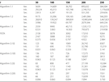
Table 1 Computational results for Example 5.1 with (N,M) = (100, 50)
J 50 100 150 200 250
Algorithm 1.1 Iter. 3263 90,378 297,135 65,795 31,655
Inlt. 13,748 377,483 864,321 172,925 82,979
Sec. 2.188 36.672 110.563 25.500 13.781
Algorithm 1.2 Iter. 8732 194,940 434,539 82,993 43,689
Inlt. 46,182 1,069,758 1,327,537 225,913 141,813
Sec. 6.797 106.234 189.078 38.094 23.422
Algorithm 1.3 Iter. 336 2012 4302 1327 676
Sec. 0.063 0.406 1.125 0.406 0.219
FISTA Iter. 1389 2580 3787 3260 2491
Inlt. 1397 2589 3796 3270 2501
Sec. 0.391 0.453 0.734 0.656 0.563
Algorithm 3.1(I) Iter. 199 793 4342 482 718
Inlt. 254 913 5206 1145 1148
Sec. 0.094 0.156 0.953 0.156 0.188
Algorithm 3.1(II) Iter. 152 764 2176 580 697
Inlt. 184 860 2232 604 769
Sec. 0.078 0.219 0.406 0.125 0.125
Algorithm 3.2(I) Iter. 81 2208 5704 1022 362
Inlt. 178 4680 7562 2261 846
Sec. 0.063 0.469 1.891 0.250 0.094
Algorithm 3.2(II) Iter. 65 952 2311 629 263
Inlt. 80 976 2375 653 288
Sec. 0.031 0.188 0.516 0.156 0.063
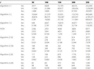
Table 2 Computational results for Example 5.1 with (N,M) = (150, 150)
J 50 100 150 200 250
Algorithm 1.1 Iter. 5639 14,609 36,702 895,632 364,304
Inlt. 29,524 43,313 107,748 2,740,752 1,179,620
Sec. 2.813 6.297 19.125 551.250 259.656
Algorithm 1.2 Iter. 9175 33,306 109,165 2,481,066 566,203
Inlt. 28,810 139,247 389,839 10,985,694 3,467,821
Sec. 3.906 19.922 69.797 2079.344 649.234
Algorithm 1.3 Iter. 2559 9995 40,713 1,535,172 353,573
Sec. 0.531 3.063 16.563 793.875 219.938
FISTA Iter. 2158 3078 3092 17,010 9264
Inlt. 2167 3088 3102 17,021 9275
Sec. 0.375 0.656 0.797 4.922 2.984
Algorithm 3.1(I) Iter. 123 186 1069 26,742 8307
Inlt. 131 690 1779 32,790 15,519
Sec. 0.031 0.063 0.359 7.750 5.141
Algorithm 3.1(II) Iter. 136 171 726 17,575 3765
Inlt. 160 187 807 18,007 3813
Sec. 0.063 0.125 0.188 5.047 1.922
Algorithm 3.2(I) Iter. 83 808 477 27,199 10,584
Inlt. 182 1713 1140 31,301 12,084
Sec. 0.063 0.125 0.147 13.078 5.563
Algorithm 3.2(II) Iter. 43 235 297 15,515 7331
Inlt. 66 251 322 15,839 7520
[image:23.595.118.477.407.677.2]Table 3 Computational results for Example 5.1 with (N,M) = (200, 250)
J 50 100 150 200 250
Algorithm 1.1 Iter. 3477 6828 15,749 48,555 255,440
Inlt. 11,943 21,084 60,677 336,456 1,326,061
Sec. 1.688 3.844 12.672 67.453 334.891
Algorithm 1.2 Iter. 10,464 21,319 32,055 122,743 483,468
Inlt. 30,876 86,575 162,387 420,341 2,185,371
Sec. 5.281 16.063 32.156 111.891 600.625
Algorithm 1.3 Iter. 648 6647 16,810 44,817 132,873
Sec. 0.188 2.781 9.500 32.734 118.203
FISTA Iter. 2346 2931 4040 3804 6977
Inlt. 2355 2941 4051 3815 6989
Sec. 0.500 0.750 1.250 1.344 3.141
Algorithm 3.1(I) Iter. 109 236 343 814 2077
Inlt. 151 278 415 975 2518
Sec. 0.031 0.094 0.188 0.344 7.078
Algorithm 3.1(II) Iter. 168 188 262 756 1106
Inlt. 180 200 268 792 1142
Sec. 0.063 0.109 0.125 0.218 0.438
Algorithm 3.2(I) Iter. 117 168 818 1718 1725
Inlt. 128 222 986 2000 2408
Sec. 0.063 0.063 0.438 1.063 1.281
Algorithm 3.2(II) Iter. 82 83 373 582 1240
Inlt. 98 108 400 644 1285
[image:24.595.119.479.393.596.2]Sec. 0.031 0.078 0.199 0.406 0.563
Figure 1 Numbers of projections with (N,M) = (100, 50).
We takeL0= 13,η= 2 anda= 7 for FISTA with backtracking (see [21]). For compari-son, the same random values are taken in each test for different algorithms.
The numerical results are listed in Tables 1, 2, 3 and Figures 1-6, from which we can get some conclusions:
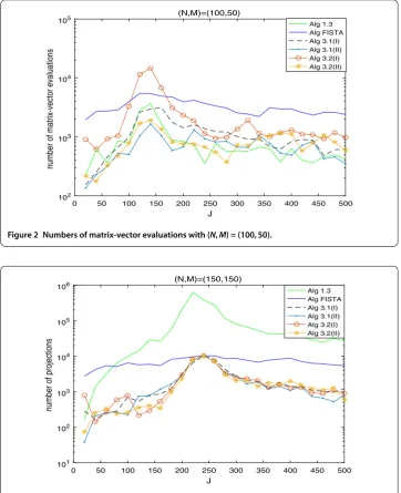
Figure 2 Numbers of matrix-vector evaluations with (N,M) = (100, 50).
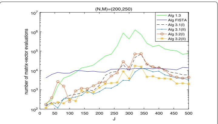
Figure 3 Numbers of projections with (N,M) = (150, 150).
(2) The numbers of projections and matrix-vector evaluations that Algorithms 1.3, 3.1 and 3.2 need are close whenM,Nare small. However, the numbers of projections and matrix-vector evaluations that Algorithms 3.1 and 3.2 need are less than those of Algorithm 1.3 asM,Nbecome bigger.
(3) In Figures 1, 3 and 5, the number of projections of Algorithm 3.1(I) and (II) (or Algorithm 3.2) is close although the iteration number of Algorithm 3.1(II) is less than that of Algorithm 3.1(I). The reason is that two projections are needed in Algorithm 3.1(II) while one projection is needed in Algorithm 3.1(I) per each iteration.
Figure 4 Numbers of matrix-vector evaluations with (N,M) = (150, 150).
Figure 5 Numbers of projections with (N,M) = (200, 250).
(5) From Figures 1-5, it is observed that there exist peak values for Algorithms 1.3, 3.1 and 3.2, while FISTA has no peak values and is better than Algorithms 1.3, 3.1 and 3.2 near the peak values for some cases. However, for the other values ofM,N,J, Algorithms 3.1 and 3.2 behave better than FISTA.
6 Conclusion
Figure 6 Numbers of matrix-vector evaluations with (N,M) = (200, 250).
A numerical experiment is provided to illustrate that, except for FISTA, Algorithms 1.3, 3.1 and 3.2 have peak values. It is thus natural to combine our methods with inertial effects. This is one of our future research topics.
Acknowledgements
The authors are supported by the National Natural Science Foundation of China (No. 71602144) and Open Fund of Tianjin Key Lab for Advanced Signal Processing (No. 2016ASP-TJ01). The authors would like to thank two anonymous referees for their careful reading of an earlier version of this paper and constructive suggestions. In particular, one referee gave us very valuable comments on the numerical experiments, and we added Section 3.2 under his opinions, which enabled us to improve the paper greatly.
Competing interests
The authors declare that they have no competing interests.
Authors’ contributions
All authors contributed equally to the writing of this paper. All authors read and approved the final manuscript.
Publisher’s Note
Springer Nature remains neutral with regard to jurisdictional claims in published maps and institutional affiliations.
Received: 11 April 2017 Accepted: 15 December 2017
References
1. Moudafi, A: Alternating CQ-algorithm for convex feasibility and split fixed-point problem. J. Nonlinear Convex Anal.
15(4), 809-818 (2014)
2. Attouch, H, Cabot, H, Frankel, F, Peypouquet, J: Alternating proximal algorithms for constrained variational inequalities: application to domain decomposition for PDE’s. Nonlinear Anal.74(18), 7455-7473 (2011) 3. Attouch, H, Bolte, J, Redont, P, Soubeyran, A: Alternating proximal algorithms for weakly coupled minimization
problems: applications to dynamical games and PDEs. J. Convex Anal.15, 485-506 (2008)
4. Censor, Y, Bortfeld, T, Martin, B, Trofimov, A: A unified approach for inversion problems in intensity-modulated radiation therapy. Phys. Med. Biol.51, 2353-2365 (2006)
5. Attouch, H: Alternating minimization and projection algorithms. From convexity to nonconvexity. Communication in Instituto Nazionale di Alta Matematica Citta Universitaria - Roma, Italy, 8-12 June (2009)
6. Moudafi, A: A relaxed alternating CQ-algorithm for convex feasibility problems. Nonlinear Anal.79, 117-121 (2013) 7. Tian, D, Shi, L, Chen, R: Iterative algorithm for solving the multiple-sets split equality problem with split self-adaptive
step size in Hilbert spaces. J. Inequal. Appl.2016, 34 (2016)
8. Dong, QL, He, SN: Modified projection algorithms for solving the split equality problems. Sci. World J.2014, 328787 (2014)
9. Dong, QL, He, SN: Self-adaptive projection algorithms for solving the split equality problems. Fixed Point Theory
18(1), 191-202 (2017)