2019 International Conference on Computer Science, Communications and Multimedia Engineering (CSCME 2019) ISBN: 978-1-60595-650-3
Research on Cold Chain Logistics Distribution Routing Algorithm Model
Based on Customer Satisfaction
Cun-hui DENG
1, You-shi HE
1and Jin-hai LI
21Jiangsu University, Zhenjiang
2Taizhou University, Taizhou
Keywords: Customer satisfaction, Cold chain logistics, Vehicle path, Genetic algorithm.
Abstract. In view of the characteristics of cold chain logistics different from ordinary products and the competition within the industry, the distribution of chilled and frozen foods requires the use of refrigerated vehicles, and the cost of transportation and distribution is high. In the study of cold chain logistics, in order to more fully reflect customer satisfaction, this paper establishes a multi-objective optimization model with the lowest distribution cost and the shortest time; then introduces the customer satisfaction index and establishes a multi-objective optimization model of customer satisfaction. Linear processing transforms multiple goals into single-objective optimization problems.
Introduction
In 2018, the "Proposal on Accelerating the Commercialization of Fruit and Vegetable Production and the Innovation of Cold Chain Logistics to Promote the Development of Modern Fruit and Vegetable Industry" proposed strengthening the construction of scientific and technological teams and supporting conditions, and improving the technological innovation capability of commercialization of fruit and vegetable production and cold chain logistics. This shows that China attaches importance to accelerating cold chain logistics.
Problem Description and Model Construction
Problem Description
Related variable description
A—Customer collection,Set the total number of customers to N, A
0,1, 2,3, ,N
, Use k torepresent specific customers, kA, k=0 Representative transportation center;
j P
—k Customer's total receipt and shipping weight;
B—Total number of vehicles, Set the total number of vehicles to M, B
1, 2,3, ,M
, Use u toindicate a specific vehicle, uB;
W—Capacity per car, tons;
—Freshness loss coefficient of the delivery vehicle during transportation, km h/ ;
—Refrigeration energy consumption coefficient of loading and unloading truck, yuan/km;
—Refrigeration energy consumption coefficient of the delivery vehicle during transportation,
yuan/km;
u
c —Fixed operating cost of a car, yuan;
V —Average speed of the vehicle, km h/ ;
0
c —Transportation cost per kilometer, yuan /km
;
ij T
—Delivery u time from customer i to customer j, h;
auk
T —When the vehicle u arrives at the customer k;
duk
T —When the vehicle u leaves the customer k;
—Unit weight loading and unloading time factor , ton/h;
0
e —Customer's minimum satisfaction;
Defining variables xijuandxju, The meaning of the two is as follows:
;
Target Model Establishment
Cost Model. The fixed cost can be approximated as:
1 1 M u u C c
(1)To simplify the analysis, assume that the cost is proportional to the distance traveled by the vehicle, and its analytical expression is:
2 0
1 0 0 M N N
ij iju u i j
C
c D x
(2)
this paper introduces the energy consumption coefficient of loading and unloading refrigeration
and transportation refrigeration coefficient . Therefore, the cost of refrigeration can be
approximated as:
3
1 0 0
+
M N N
ij iju j iju u i j
C
D x
P x
(3)Therefore the total cost can be expressed as:
0 1 1 0 0
1 0 0
+ +
+
M M N N
u ij iju
u u i j
M N N
ij iju j iju u i j
C c c D x
D x P x
(4)The constraints on the variables xiju
are shown in equations (5)~(8).
0 1 1 M N ju u j x M
(5)
and
1 1, 2, ,
M N iju
x j N i j
0 0
1 1
=1
N N
i u ju
i j
x x u B
(7)The total quantity of goods on each transport route must not exceed the load per vehicle, therefore:
0 0 N N
i iju i i
P
x
M
(8) Equation (6) indicates that the total number of paths cannot exceed the total number of vehicles; Equation (7) indicates that a customer is served by only one truck; Equation (8) indicates that the starting point and starting point of each path are distribution centers.
Time Model. The unit weight loading and unloading time factor is introduced. The total time of delivery can be expressed as:
1 0 0 1 0 0 M N N M N N
ij iju j iju u i j u i j
T
T x
P x
(9)Where, for the time between the delivery of the car from the customer to the customer, the analytical expression is:
In the middle, Tij For delivery vehicles u Time from customer i to customer j, Its analytical
expression is:
=
ijij
D
T
V
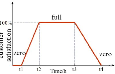
(10)Satisfaction Model. When the time is less than t1 and greater than t4, the satisfaction is 0, and the function of satisfaction and time is as shown in equation (11).
Introducing satisfaction correction factor , Indicates the customer’s satisfaction with the
freshness of the goods, The expression is as shown in equation (7), and FIG. 2 is a graph of the satisfaction correction coefficient as a function of time.
=1-
t
k
(11)Where tk is the time it takes for the truck to reach the customer k from the distribution center, ie
the Tauk mentioned in the previous paragraph, ie
=
k auk
T
T
(12)The difference between Tauk and Tauk is the total time that the truck is serviced at customer k.
The constraint relationship between the two is:
-duk auk k
Figure 1. Customer satisfaction changes over time.
1
1 2 1 1 2
2 3
4 4 3 3 4
4
0 0
/ 1
/ 0
k
k k
k k k
k k
k t t t t t t t t t t t t e t
t t t t t t t t t
[image:4.595.73.441.228.512.2](14)
Figure 2. Customer satisfaction changes over time.
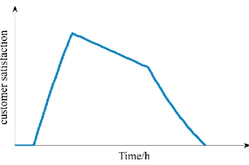
Multiplying the satisfaction calculated by equation (11) by the correction factor can obtain
the overall satisfaction of the customer. The analytical expression is:
=
k k k
e t
e t (15) The corrected customer satisfaction curve over time is shown in Figure 3. Therefore customer satisfaction is:
1
M
k k k
E e t
Figure 3. Customer satisfaction changes over time.
Multi-objective Optimization Model with Minimum Distribution Cost and Minimum Delivery Time
The objective function is infinitely tempered by the range method.
y’j=(yj-min yj)/(max yj-min yj) (17) In the formula, the variable yj is subjected to the tempering tempering process to obtain the variable y'j, y'j is between [0, 1], and C' and T' are the objective functions obtained by the above-described non-classification processing of C and T.
You need to set the weight vector P=(a,b), where a+b=1, a,b between the interval [0,1], then Q=aC+bT, he weight variable P=(0.8, 0.2), therefore, the comprehensive objective function can be obtained as
minQ|Q =0.8C’+0.2T’ (18) After linear weighting, the multi-objective optimization problem is transformed into the single-objective problem shown in (18).
In Conclusion
This paper combines customer satisfaction with cold chain logistics path distribution, but still has the following shortcomings: on the one hand, it does not combine the characteristics of cold chain logistics; on the other hand, this paper does not consider the case verification of model algorithm, not comprehensive enough, etc. The direction.
References
[1] Shi Wei, Jia Bonian. Optimal Distribution Path Planning Problem in Smart Logistics [J/OL]. Electronic Technology and Software Engineering, 2019(05): 255.
[2] Jing Jing, Zhou Wei, Hu Yuqun. Selection of urban fresh logistics distribution route with hard time window under time-varying road network [J/OL]. Highway and Motor Transport, 2019(01): 65-68.
[4] Yuan Hongbin, Yang Yan. Study on the Optimization of Vegetable Cold Chain Logistics Distribution Path Based on Customer Satisfaction[J]. Modern Trade and Industry, 2018, 39(07):63-64.
[5] Li Changbing, Wang Erjing, Yuan Jiabin. Study on the Optimization of Logistics Distribution Routing of Fresh Agricultural Products under the Environment of Internet of Things[J]. Commercial Research, 2017(04):1-9.
[6] He Runxin, Gonzalez Humberto. Numerical Synthesis of Pontryagin Optimal Control Minimizers Using Sampling-Based Methods[C]//IEEE 56th Annual Conference on Decision and Control (CDC). Melbourne, Australia: IEEE CDC, 2017:733-738