R E S E A R C H
Open Access
Self-adaptive subgradient extragradient
method with inertial modification for solving
monotone variational inequality problems
and quasi-nonexpansive fixed point problems
Ming Tian
1*and Mengying Tong
1*Correspondence: [email protected] 1College of Science, Civil Aviation
University of China, Tianjin, China
Abstract
In this paper, we introduce a new algorithm with self-adaptive method for finding a solution of the variational inequality problem involving monotone operator and the fixed point problem of a quasi-nonexpansive mapping with a demiclosedness property in a real Hilbert space. The algorithm is based on the subgradient
extragradient method and inertial method. At the same time, it can be considered as an improvement of the inertial extragradient method over each computational step which was previously known. The weak convergence of the algorithm is studied under standard assumptions. It is worth emphasizing that the algorithm that we propose does not require one to know the Lipschitz constant of the operator. Finally, we provide some numerical experiments to verify the effectiveness and advantage of the proposed algorithm.
Keywords: Variational inequality problem; Fixed point problem; Extragradient method; Subgradient extragradient method; Inertial method; Self-adaptive method
1 Introduction
Throughout this paper, letHbe a real Hilbert space with the inner product·,·and norm · . LetCbe a nonempty, closed and convex subset ofH. LetNandRbe the sets of positive integers and real numbers, respectively.
The variational inequality problem (VIP) is the problem to find a pointx∗∈Csuch that
Ax∗,x–x∗≥0, ∀x∈C. (1)
The solution set of VIP is denoted byVI(C,A). The variational inequality problem is an important branch of the nonlinear problem and it has received a lot of attentions by many authors in recent years (see [1–3] and the references therein). Under appropriate condi-tions, there are two general approaches for solving the variational inequality problem, one is the regularized method and the other is the projection method. Now, we mainly study the projection method.
For every pointx∈H, there exists a unique point inCsuch that
x–PCx=infx–y:y∈C,
wherePC:H→Cis called the metric projection fromHintoC.
We know that the variational inequality problem can be turned into the fixed point prob-lem, which means (1) is equivalent to
x∗=PC(I–λA)x∗, (2)
wherePC:H→Cis the metric projection andλ> 0. Thus we generate{xn}in the follow-ing manner:
xn+1=PC(I–λA)xn. (3)
This simple algorithm is an extension of the projection gradient method. However, the convergence of this method requires a slight assumption that the operatorA:H→His strongly monotone or inverse strongly monotone.
To avoid this strong assumption, Korpelevich [4] proposed an algorithm which was called the extragradient method:
⎧ ⎨ ⎩
yn=PC(xn–λAxn),
xn+1=PC(xn–λAyn),
(4)
for eachn= 1, 2, . . . , whereλ∈(0, 1/L). At the beginning, this method was used to solve saddle point problems. Soon, this method was extended to Euclidean spaces and Hilbert spaces. In particular, this method only requires that the operatorAis monotone andL -Lipschitz continuous in a Hilbert space. IfVI(C,A)=∅, the sequence{xn}generated by
(4) converges weakly to an element ofVI(C,A).
However, the extragradient method needs to calculate two projections fromHonto the closed convex setCand it is applicable to the case thatPChas a closed form which means thatPChas an explicit expression. In fact, in some cases, the projection onto the nonempty closed convex subsetCmight be difficult to calculate. To overcome this drawback, it has received great attentions by many authors who had improved it in various ways.
To our knowledge, there were four kinds of methods to overcome this drawback. The first one was the modification of the extragradient method by Tseng [5] who proposed it in 2000 with the following remarkable scheme:
⎧ ⎨ ⎩
yn=PC(xn–λAxn),
xn+1=yn–λ(Ayn–Axn),
(5)
2011: ⎧ ⎪ ⎪ ⎨ ⎪ ⎪ ⎩
yn=PC(xn–λAxn),
Tn={w∈H| xn–λAxn–yn,w–yn ≤0},
xn+1=PTn(xn–λAyn),
(6)
whereAis monotone,L-Lipschitz continuous andλ∈(0, 1/L). The key operation of the subgradient extragradient method replaces the second projection ontoCof the extragra-dient method by a projection onto a special constructible half-space, which significantly reduces the difficulty of calculations.
Before explaining the third method, let us take a look at the inertial method. In 2001, Al-varez and Attouch [7] applied the inertial technique to obtain an inertial proximal method to solve the problem of finding zero of a maximal monotone operator, which works as fol-lows:
findxn+1∈H, such that 0∈λnA(xn+1) +xn+1–xn–θn(xn–xn–1),
wherexn–1,xn∈H,θn∈[0, 1) andλn> 0. It also can be written in the following form:
xn+1=JλAn
xn+θn(xn–xn–1)
, (7)
where JA
λn is the resolvent ofA with parameter λn and the inertia is induced by the
termθn(xn–xn–1). Recently, considerable interest has been shown in studying the
iner-tial method by many authors. They constructed fast iterative algorithms by using ineriner-tial method. The third method which was studied by Q.L. Dong et al. [8] in 2017:
⎧ ⎪ ⎪ ⎪ ⎪ ⎪ ⎨ ⎪ ⎪ ⎪ ⎪ ⎪ ⎩
wn=xn+αn(xn–xn–1),
yn=PC(wn–λAwn),
d(wn,yn) = (wn–yn) –λ(Awn–Ayn),
xn+1=wn–γ βnd(wn,yn),
(8)
for eachk≥1, whereγ ∈(0, 2),λ> 0,
βn:= ⎧ ⎨ ⎩
ϕ(wn,yn)/d(wn,yn)2, ifd(wn,yn)= 0,
0, ifd(wn,yn) = 0,
ϕ(wn,yn) =wn–yn,d(wn,yn).
This algorithm incorporate the inertial terms in the projection and contraction algorithm, which does not need the summability condition for the sequence. The fourth one was a self-adaptive algorithm which was based on Tseng’s extragradient method [9] and it was proposed by Duong Viet Thong and Dang Van Hieu [9] in 2017. The algorithm is described as follows.
Algorithm 1A SA-Tseng’s EGM for monotone variational inequality problem Step 1: Choosex0∈H,γ > 0,l∈(0, 1),μ∈(0, 1).
Step 2: Given the current iteratexn, compute
yn=PC(xn–λnAxn),
whereλnis chosen to be the largestλ∈ {γ,γl,γl2, . . .}satisfying
λAxn–Ayn ≤μxn–yn.
Ifyn=xn, then stop andxnis the solution of the variational inequality problem. Otherwise,
Step 3: Compute the new iteratexn+1via the following iterate formula:
xn+1=yn–λn(Ayn–Axn).
Setn:=n+ 1 and return to Step 2.
∅, the sequences{xn}generated by (5), (6), (8) and Algorithm1all converge weakly to an
element ofVI(C,A). For Algorithm1, it does not require to know the Lipschitz constant, but the step size may involve computation of additional projections.
In 2016, Mainge and Gobinddass [10] gotxn+1by the following algorithm:
⎧ ⎨ ⎩
yn=xn+θn(xn–xn–1),
xn+1=PC(xn–λnAyn),
(9)
whereθn=δλλnn–1,λnkn≤εδ( √
2 – 1),λn≤kλn–1(δ+λλnn–1–2) 1
2,{λn} ⊂[μ,ν] and
kn:= ⎧ ⎨ ⎩
Ayn–Ayn–1
yn–yn–1 , ifyn–yn–1= 0, 0, ifyn–yn–1= 0.
In this iterative algorithm, it does not require either additional projection for the determi-nation of the step-sizes or the knowledge of the Lipschitz constant of the operator.
The fixed point problem is the problem to findx∗∈Hsuch that
Tx∗=x∗, (10)
where x∗ is called a fixed point ofT :H→H. The set of fixed points ofT is denoted byFix(T). Recently, many iterative methods have been proposed (see [6,11–21] and the references therein) for finding a common element ofFix(T) andVI(C,A) in a real Hilbert space.
point problem of a quasi-nonexpansive mapping with a demiclosedness property in a real Hilbert space. Then the weak convergence theorem will be proved in Sect.3.
This paper is organized as follows. In Sect.2, we list some lemmas which will be used for further proof. In Sect.3, we proposed a new algorithm, then the weak convergence the-orem is analyzed. In Sect.4, we give some numerical examples to illustrate the efficiency and advantage of our algorithm.
2 Preliminaries
In this section, we introduce some lemmas which will be used in this paper. AssumeHis a real Hilbert space andCis a nonempty closed convex subset ofH. In the following of the paper, we use the symbolxn→xto denote the strong convergence of the sequence{xn}to
xasn→ ∞and use the symbolxnxto denote the weak convergence of the sequence
{xn}toxasn→ ∞. If there exists a subsequence{xni}of{xn}converging weakly to a point z, thenzis called a weak cluster point of{xn}and the set of all weak cluster points of{xn}
is denoted byωw(xn).
Lemma 2.1([22]) Let H be a real Hilbert space,for each x,y∈H andλ∈R,we have
(i) x+y2=x2+y2+ 2x,y;
(ii) λx+ (1 –λ)y2=λx2+ (1 –λ)y2–λ(1 –λ)x–y2.
In the following, we gather some characteristic properties ofPC.
Lemma 2.2([23]) Let H be a real Hilbert space and C be a nonempty closed subset of H.
Then
(i) PCx–PCy2≤ x–y,PCx–PCy,∀x,y∈H;
(ii) x–PCx2+y–PCx2≤ x–y2,∀x∈H,y∈C.
Lemma 2.3 Let H be a real Hilbert space and C be a nonempty closed subset of H.Given x∈H and z∈C,then z=PCx if and only if there hold the inequalityx–z,y–z ≤0, ∀y∈C.
Next, we present some concepts of an operator.
Definition 2.4([24]) An operatorA:H→His said to be: (i) monotone, if
x–y,Ax–Ay ≥0, ∀x,y∈H;
(ii) L-Lipschitz continuous withL> 0, if
Ax–Ay ≤Lx–y, ∀x,y∈H;
(iii) nonexpansive, if
(iv) quasi-nonexpansive, if
Ax–p ≤ x–p, ∀x∈H,p∈Fix(A),
whereFix(A)=∅.
Remark2.5 ([25]) It is well that every nonexpansive mapping with a nonempty set of fixed point is quasi-nonexpansive. However, a quasi-nonexpansive mapping may not be a non-expansive mapping.
Lemma 2.6([23]) Assume that T:H→H is a nonlinear operator withFix(T)=∅.Then I–T is said to be demiclosed at zero if for any{xn}in H,the following implication holds:
xnx and (I–T)xn→0⇒x∈Fix(T).
Remark2.7 We know that the Lemma2.6is clearly established when the operatorT is nonexpansive. However, there exists a quasi-nonexpansive mapping T butI–T is not demiclosed at zero. Therefore, in this paper, we need to emphasize thatT :H→His a quasi-nonexpansive mapping such thatI–Tis demiclosed at zero.
Example1 LetHbe the line real andC= [0,32]. Define the operatorTonCby
Tx=
⎧ ⎨ ⎩ x
2, ifx∈[0, 1],
xcos2πx, ifx∈(1,32].
Indeed, it is easy to see thatFix(T) ={0}. On the one hand, for anyx∈[0, 1], we have
|Tx– 0|=x 2– 0
≤ |x– 0|.
On the other hand, for anyx∈(1,32], we have
|Tx– 0|=|xcos2πx– 0|=|xcos2πx– 0| ≤ |x|=|x– 0|.
Thus, the operatorTis quasi-nonexpansive.
By taking{xn} ⊂(1,32] andxn→1 asn→ ∞, we have
(I–T)xn=|xn–Txn|=|xn–xncos2πxn|=|xn| · |1 –cos2πxn| →0 (n→ ∞).
But 1 /∈Fix(T), soI–T is not demiclosed at zero.
Lemma 2.8([7]) Let{ϕn},{δn}and{αn}be sequences in[0, +∞)such that
ϕn+1≤ϕn+αn(ϕn–ϕn–1) +δn, ∀n≥1,
+∞
n=1
δn< +∞,
(i) +n=1∞[ϕn–ϕn–1]+< +∞,where[t]+:=max{t, 0};
(ii) there existsϕ∗∈[0, +∞)such thatlimn→+∞ϕn=ϕ∗.
Lemma 2.9([26]) Let A:H→H be a monotone and L-Lipschitz continuous mapping on C.Let S=PC(I–μA),whereμ> 0.If{xn}is a sequence in H satisfying xnq and xn–Sxn→0,then q∈VI(C,A) =Fix(S).
Lemma 2.10([27]) Let C be a nonempty closed and convex subset of a real Hilbert space H and{xn}be a sequence in H.The following two properties hold:
(i) limn→∞xn–xexists for eachx∈C;
(ii) ωw(xn)⊂C.
Then the sequence{xn}converges weakly to a point in C.
3 Main results
In this section, we propose a new iterative algorithm with self-adaptive method for solving monotone variational inequality problems and quasi-nonexpansive fixed point problems in a Hilbert space. Meanwhile, we combine subgradient extragradient method and inertial modification for the algorithm. Under the assumptionFix(T)∩VI(C,A)=∅, we prove the weak convergence theorem. LetHbe a real Hilbert space. LetCbe a nonempty closed convex subset inH. LetA:H→Hbe a monotone andL-Lipschitz continuous operator. In particular, the information of the Lipschitz constantLdoes not require to be known. LetT:H→Hbe a quasi-nonexpansive mapping such thatI–T is demiclosed at zero. The algorithm is described as follows.
Before giving the theorem and its proof, we propose several useful lemmas firstly.
Lemma 3.1 The sequence{λn}generated by Algorithm2is a monotonically decreasing sequence,and its lower bound ismin{μL,λ0}.
Proof It is obvious that the sequence{λn}is a monotonically decreasing sequence.
SinceAisL-Lipschitz continuous withL> 0, we have
Axn–Ayn ≤Lxn–yn.
In the case ofAxn–Ayn= 0, we have
μxn–yn
Axn–Ayn≥
μ
L.
Clearly, the lower bound of the sequence{λn}ismin{μL,λ0}.
Lemma 3.2 If wn=yn=xn+1,then wn∈Fix(T)∩VI(C,A).
Proof Ifwn=yn, we havewn∈VI(C,A).
Algorithm 2A ISA-SEGM for monotone variational inequality problem Step 1: Choosex0,x1∈H,μ∈(0, 1),λ0> 0.
Step 2: Setwn=xn+αn(xn–xn–1), compute
yn=PC(wn–λnAwn).
Step 3: Compute
zn=PTn(wn–λnAyn),
whereTn={x∈H|wn–λnAwn–yn,x–yn ≤0}.
Step 4: Compute
xn+1= (1 –βn)wn+βnTzn
and
λn+1:=
⎧ ⎨ ⎩
min{ μxn–yn
Axn–Ayn,λn}, ifAxn–Ayn= 0,
λn, otherwise.
Ifwn=yn=xn+1, thenwn∈Fix(T)∩VI(C,A).
Setn:=n+ 1 and return to Step 2.
On the other hand, ifwn=yn=xn+1, byxn+1= (1 –βn)wn+βnTzn, we have
wn= (1 –βn)wn+βnTwn,
through deformation, we can getTwn=wn, which meanswn∈Fix(T).
Therefore,wn∈Fix(T)∩VI(C,A).
Lemma 3.3 Let{zn}be a sequence generated by Algorithm2,then,for all p∈VI(C,A),and for n sufficiently large,we have
zn–p2≤ wn–p2– (1 –μγ)yn–wn2
– (1 –μγ)zn–yn2– 2λnAp,yn–p. (11)
Proof Sincep∈VI(C,A) andVI(C,A)⊂C⊂Tn, we have
zn–p2=PTn(wn–λnAyn) –p
2
≤PTn(wn–λnAyn) –PTnp,wn–λnAyn–p
=zn–p,wn–λnAyn–p
= 1
2zn–p
2+1
2wn–λnAyn–p
2–1
2zn–wn+λnAyn
2
= 1
2zn–p
2+1
2wn–p
2+1
2λ
2
–wn–p,λnAyn–1
2zn–wn
2–1
2λ
2
nAyn2
–zn–wn,λnAyn
= 1
2zn–p
2+1
2wn–p
2–1
2zn–wn
2–z
n–p,λnAyn.
It implies that
zn–p2≤ wn–p2–zn–wn2– 2zn–p,λnAyn.
Because the operatorAis monotone andλn> 0, we have
2λnAyn–Ap,yn–p ≥0.
So
zn–p2≤ wn–p2–zn–wn2– 2zn–p,λnAyn
+ 2λnAyn–Ap,yn–p
=wn–p2–zn–wn2+ 2λn
Ayn–Ap,yn–p
–zn–p,Ayn
=wn–p2–zn–wn2+ 2λn
Ayn,yn–p–Ap,yn–p
–zn–p,Ayn
=wn–p2–zn–wn2+ 2λn
Ayn,yn–zn–Ap,yn–p
=wn–p2–zn–wn2+ 2λnAyn–Awn,yn–zn
+ 2λnAwn,yn–zn– 2λnAp,yn–p.
Since{λn}is a monotonically decreasing sequence, the limit of{λn}exists andλλnn+1≥1. We denoteλ=limn→∞λn. Therefore, we havelimn→∞=λλnn+1= 1. We haveμ∈(0, 1),
1
μ>
1, letγ=1+ 1
μ
2 , 1 <γ < 1
μ. Therefore,∃N∈N,∀n>N, λn
λn+1<γ. Therefore, 1 –μγ < 1.
2λnAyn–Awn,yn–zn ≤2λnyn–zn · Ayn–Awn
≤2λnyn–zn ·
μ λn+1
yn–wn
≤2μγyn–zn · yn–wn
≤μγyn–zn2+μγyn–wn2.
Sincezn∈Tn, we have
wn–λnAwn–yn,zn–yn ≤0.
So
2λnAwn,yn–zn ≤2yn–wn,zn–yn
Therefore
zn–p2≤ wn–p2–zn–wn2+ 2λnAyn–Awn,yn–zn
+ 2λnAwn,yn–zn– 2λnAp,yn–p
≤ wn–p2–zn–wn2+μγyn–zn2+μγyn–wn2
+zn–wn2–yn–wn2–zn–yn2– 2λnAp,yn–p
=wn–p2– (1 –μγ)yn–wn2– (1 –μγ)zn–yn2
– 2λnAp,yn–p.
Theorem 3.4 Assume that the sequence{αn}is non-decreasing such that0≤αn≤α≤14 and the sequence{βn}is a sequence of real numbers such that0 <β≤βn≤ 12.Then the sequence{xn}generated by Algorithm2converges weakly to an element ofFix(T)∩VI(C,A).
Proof Letp∈Fix(T)∩VI(C,A).
From Lemma3.3, we have∃N≥0,∀n>N,zn–p ≤ wn–p.
SinceTis quasi-nonexpansive, by Lemma2.1, we have∀n>N
xn+1–p2=(1 –βn)wn+βnTzn–p2
=(1 –βn)(wn–p) +βn(Tzn–p)
2
= (1 –βn)wn–p2+βnTzn–p2–βn(1 –βn)Tzn–wn2
≤(1 –βn)wn–p2+βnzn–p2–βn(1 –βn)Tzn–wn2
≤(1 –βn)wn–p2+βnwn–p2–βn(1 –βn)Tzn–wn2
=wn–p2–βn(1 –βn)Tzn–wn2. (12)
Sincexn+1= (1 –βn)wn+βnTzn, we can write it as
Tzn–wn= 1 βn
(xn+1–wn). (13)
Combining (12) and (13), withβn≤12, we have
xn+1–p2≤ wn–p2–
1 –βn
βn
xn+1–wn2
≤ wn–p2–xn+1–wn2. (14)
Besides,
wn–p2=xn+αn(xn–xn–1) –p 2
=(1 +αn)(xn–p) –αn(xn–1–p)2
= (1 +αn)xn–p2–αnxn–1–p2
and
xn+1–wn2 =xn+1–
xn+αn(xn–xn–1)2
=xn+1–xn2+αn2xn–xn–12– 2αnxn+1–xn,xn–xn–1
≥ xn+1–xn2+αn2xn–xn–12
– 2αnxn+1–xn · xn–xn–1
≥ xn+1–xn2+αn2xn–xn–12–αnxn+1–xn2
–αnxn–xn–12
= (1 –αn)xn+1–xn2+
αn2–αn
xn–xn–12. (16)
Combining (14), (15), (16), and{αn}being non-decreasing, we obtain
xn+1–p2≤(1 +αn)xn–p2–αnxn–1–p2+αn(1 +αn)xn–xn–12
– (1 –αn)xn+1–xn2–
α2n–αn
xn–xn–12
= (1 +αn)xn–p2–αnxn–1–p2– (1 –αn)xn+1–xn2
+αn(1 +αn) –
αn2–αn
xn–xn–12
= (1 +αn)xn–p2–αnxn–1–p2– (1 –αn)xn+1–xn2
+ 2αnxn–xn–12
≤(1 +αn+1)xn–p2–αnxn–1–p2– (1 –αn)xn+1–xn2
+ 2αnxn–xn–12. (17)
Therefore,
xn+1–p2–αn+1xn–p2+ 2αn+1xn+1–xn2
≤ xn–p2–αnxn–1–p2+ 2αnxn–xn–12
+ 2αn+1xn+1–xn2– (1 –αn)xn+1–xn2
=xn–p2–αnxn–1–p2+ 2αnxn–xn–12
+ (2αn+1– 1 +αn)xn+1–xn2. (18)
PutΓn:=xn–p2–αnxn–1–p2+ 2αnxn–xn–12.
From (18), we obtain
Γn+1–Γn≤(2αn+1– 1 +αn)xn+1–xn2. (19)
We have 0≤αn≤α≤14, –(2αn+1– 1 +αn)≥14.
SoΓn+1–Γn≤–δxn+1–xn2≤0, whereδ=14, which implies that the sequence{Γn}is
Besides,
Γn=xn–p2–αnxn–1–p2+ 2αnxn–xn–12
≥ xn–p2–αnxn–1–p2 (20)
and
Γn+1 =xn+1–p2–αn+1xn–p2+ 2αn+1xn+1–xn2
≥–αn+1xn–p2. (21)
Therefore,
xn–p2≤αnxn–1–p2+Γn
≤αxn–1–p2+Γ1
≤. . .
≤αnx0–p2+
1 +· · ·+αn–1Γ1
≤αnx0–p2+
Γ1
1 –α. (22)
This implies that the sequence{xn}is bounded. Combining (21) and (22), we have
–Γn+1≤αn+1xn–p2
≤αxn–p2
≤αn+1x0–p2+
αΓ1
1 –α. (23)
From (19), we have
δ
k
n=1
xn+1–xn2≤Γ1–Γk+1
≤Γ1+αk+1x0–p2+
αΓ1
1 –α
=αk+1x0–p2+
Γ1
1 –α
≤ x0–p2+
Γ1
1 –α, (24)
which means
∞
n=1
xn+1–xn2< +∞ (25)
and
lim
Besides, sinceαn≤α, we have
xn+1–wn=xn+1–xn–αn(xn–xn–1)
≤ xn+1–xn+αnxn–xn–1
≤ xn+1–xn+αxn–xn–1. (27)
Therefore, by (26) and (27), we can obtain
xn+1–wn →0 (n→ ∞). (28)
We have
xn+1–p2≤(1 +αn)xn–p2–αnxn–1–p2– (1 –αn)xn+1–xn2
+ 2αnxn–xn–12
≤(1 +αn)xn–p2–αnxn–1–p2+ 2αnxn–xn–12. (29)
Therefore, by (29) and Lemma2.8, we have
lim
n→∞xn–p
2=l (30)
by (15), we have
lim
n→∞wn–p
2=l (31)
and we also have
lim
n→∞xn–wn
2= 0. (32)
We have
xn+1–p2≤(1 –βn)wn–p2+βnzn–p2–βn(1 –βn)Tzn–wn2
≤(1 –βn)wn–p2+βnzn–p2,
which means
zn–p2≥
xn+1–p2–wn–p2
βn
+wn–p2. (33)
Combining (30), (31) and (33), the sequence{βn}being bounded, we have
lim inf
n→∞ zn–p
2≥ lim
n→∞wn–p
2=l.
By (11), we have
lim sup
n→∞
zn–p2≤ lim
n→∞wn–p
Therefore, we have
lim
n→∞zn–p
2=l. (34)
From Lemma3.3, we can obtain∀n>N
zn–p2≤ wn–p2– (1 –μγ)yn–wn2
and
zn–p2≤ wn–p2– (1 –μγ)zn–yn2.
By (31) and (34), we have
lim
n→∞yn–wn= 0 (35)
and
lim
n→∞zn–yn= 0. (36)
So
lim
n→∞zn–wn ≤nlim→∞
zn–yn+yn–wn= 0,
which implies
lim
n→∞zn–wn= 0. (37)
Therefore, by (12), (30) and (31), we have
lim
n→∞Tzn–wn= 0. (38)
So
lim
n→∞Tzn–z ≤nlim→∞
Tzn–wn+wn–zn= 0,
which implies
lim
n→∞Tzn–zn= 0. (39)
Since {xn} is bounded, there exist a subsequence{xnk} of {xn} andq∈H such that
xnkq.
So, by (32) we haveωnkqand by (37) we haveznkq.
Sinceznk qandI–Tis demiclosed at zero, by Lemma2.6, we haveq∈Fix(T).
On the other hand, for alln∈R, we haveλn>μL. We haveωnkqand
By Lemma2.9, we haveq∈VI(C,A). Therefore,q∈Fix(T)∩VI(C,A).
By Lemma2.10, we get the conclusion that the sequence{xn}converges weakly to an element ofFix(T)∩VI(C,A).
This completes the proof.
4 Numerical experiments
In this section, we give some numerical examples to illustrate the efficiency and advantage of our algorithm in comparisons with the well-known algorithm. We compare Algorithm2
with the weakly convergent Algorithm1[19].
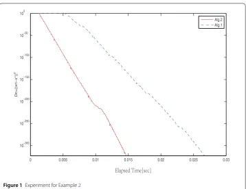
We chooseαn=14,βn=12,μ=12,λ0=17. The starting point isx0=x1= (1, 1, . . . , 1)∈Rm.
In order to show the converges of the algorithm, we illustrate the behavior of the sequence
Dn=xn–x∗2,n= 0, 1, 2, . . . , when the execution time in second elapses wherex∗is the
solution of the problem and{xn}is the sequence generated by the algorithms. Now we
introduce the examples in detail.
Example2 LetAbe a Lipschitz continuous and monotone mapping. LetT be a quasi-nonexpansive mapping. AssumeFix(T)∩VI(C,A)=∅andC= [–2, 5],H=R. LetAand
T be given by
Ax:=x+sinx,
Tx:=x 2sinx.
In the following, let us verify ifAandTmeet the requirements of the topic. First, for allx,y∈H, we have
Ax–Ay=x+sinx–y–siny ≤ x–y+sinx–siny ≤2x–y,
Ax–Ay,x–y= (x+sinx–y–siny)(x–y) = (x–y)2+ (sinx–siny)(x–y)≥0.
Therefore,Ax–Ay ≤Lx–y, whereL= 2 andAx–Ay,x–y ≥0. Therefore,Ais
L-Lipschitz continuous and monotone.
Second, forTx=x2sinx, ifx= 0 andTx=x, then we havex=x2sinx, andsinx= 2, which is impossible. Therefore, we obtainx= 0, which meansFix(T) ={0}.
For allx∈H,
Tx– 0=x 2sinx
≤x
2
<x=x– 0,
which meansTis quasi-nonexpansive. Besides, takex= 2πandy=32π, we have
Tx–Ty=2π
2 sin2π– 3π
4 sin 3π
2
=3π
4 >
2π–3π 2
=π
2,
Figure 1Experiment for Example2
Therefore,AandT meet the requirements of the topic. The numerical results for the example are shown in Fig.1.
From Fig.1, we can see that the Algorithm2converges for a shorter time than the pre-viously studied Algorithm1[19].
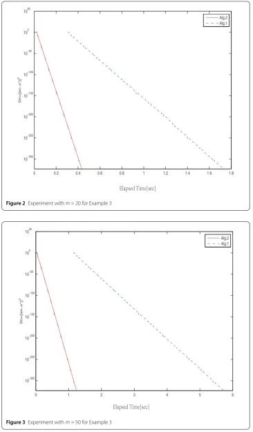
Example3 We consider the operatorT :H→H withTx= –12xand a linear operator
A:Rm→Rmin the formA(x) =Mx+q[28,29], where
M=NNT+S+D,
Nis am×mmatrix,Sis am×mskew-symmetric matrix,Dis am×mdiagonal matrix which its diagonal entries are nonnegative, andq∈Rmis a vector, thereforeMis positive definite. The feasible set is
C=x= (x1, . . . ,xm∈Rm
: –2≤xi≤5,i= 1, 2, . . . ,m}.
It is obvious thatAis monotone and Lipschitz continuous. For experiments,qis equal to zero vector, all the entries ofN,Sare generated randomly and uniformly in [–2, 2], and the diagonal entries ofDare in (0, 2).
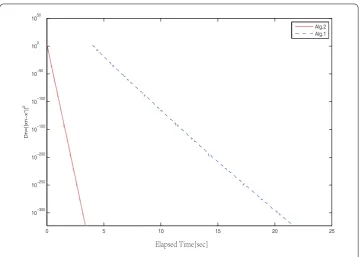
We can easily see that the solution of the algorithm in this case isx∗= 0. In order to illustrate the effectiveness of the algorithm, we show the behavior ofDnwhen execution time elapses(in second) by Figs.2,3,4inR20,R50,R100respectively.
Figure 2Experiment withm= 20 for Example3
Figure 4Experiment withm= 100 for Example3
5 Conclusion
In this paper, we introduce a new algorithm with self-adaptive method for finding a so-lution of the variational inequality problem involving monotone operator and the fixed point problem of a quasi-nonexpansive mapping with a demiclosedness property in a real Hilbert space. We combine a subgradient extragradient method and inertial modification for the algorithm. Under some suitable conditions, we have proved the weak convergence of the algorithm. In particular, it is worth emphasizing that the algorithm that we propose does not need any additional projections of the Lipschitz constant. Finally, some numeri-cal experiments are performed to verify the convergence of the algorithm and compared with previously known Algorithm1[19].
Funding
This work was supported by the Financial Funds for the Central Universities (No. 3122018L004) and Scientific research project of Tianjin Municipal Education Commission (No. 2018KJ253).
Competing interests
The authors declare that they have no competing interests.
Authors’ contributions
All the authors read and approved the final manuscript.
Publisher’s Note
Springer Nature remains neutral with regard to jurisdictional claims in published maps and institutional affiliations. Received: 29 October 2018 Accepted: 3 January 2019
References
1. Gibali, A.: Two simple relaxed perturbed extragradient methods for solving variational inequalities in Euclidean spaces. J. Nonlinear Var. Anal.2, 49–61 (2018)
3. Yao, Y.H., Chen, R.D., Xu, H.K.: Schemes for finding minimum-norm solutions of variational inequalities. Nonlinear Anal. 72, 3447–3456 (2010)
4. Korpelevich, G.M.: The extragradient method for finding saddle points and other problem. Èkon. Mat. Metody12, 747–756 (1976)
5. Tseng, P.: A modified forward-backward splitting method for maximal monotone mappings. SIAM J. Control Optim. 38, 431–446 (2000)
6. Censor, Y., Gibali, A., Reich, S.: The subgradient extragradient method for solving variational inequalities in Hilbert space. J. Optim. Theory Appl.148, 318–335 (2011)
7. Alvarez, F., Attouch, H.: An inertial proximal method for maximal monotone operators via discretization of a nonlinear oscillator with damping. Set-Valued Anal.9, 3–11 (2001)
8. Dong, Q.L., Cho, Y.J., Zhong, L.L.: Inertial projection and contraction algorithms for variational inequalities. J. Glob. Optim. (2017).https://doi.org/10.1007/s10898-017-0506-0
9. Thong, D.V., Hieu, D.V.: Weak and strong convergence theorems for variational inequality problems. Numer. Algorithms (2017).https://doi.org/10.1007/s11075-017-0412-Z
10. Mainge, P.E., Gobinddass, M.L.: Covergence of one-step projected gradient methods for variational inequalities. J. Optim. Theory Appl.171, 146–168 (2016)
11. Ceng, L.C., Yao, J.C.: Strong convergence theorem by an extragradient method for fixed point problems and variational inequality problems. Taiwan. J. Math.10, 1293–1303 (2006)
12. Iiduka, H., Takahashi, W.: Strong convergence theorems for nonexpansive mappings and inverses-strongly monotone mappings. Nonlinear Anal.61, 341–350 (2005)
13. Nadezhkina, N., Takashi, W.: Strong convergence theorem by a hybrid method for nonexpansive mappings and monotone mappings. J. Optim.16, 1230–1241 (2006)
14. Yao, Y.H., Liou, Y.C., Yao, J.C.: Iterative algorithms for the split variational inequality and fixed point problems under nonlinear transformations. J. Nonlinear Sci. Appl.10, 843–854 (2017)
15. Thong, D.V., Hieu, D.V.: An inertial method for solving split common fixed point problems. J. Fixed Point Theory Appl. 19, 3029–3051 (2017)
16. Qin, X.L., Yao, J.C.: Projection splitting algorithms for nonself operators. J. Nonlinear Convex Anal.18, 925–935 (2017) 17. Yang, Y., Yuan, Q.: A hybrid descent iterative algorithm for a split inclusion problem. J. Nonlinear Funct. Anal.2018,
Article ID 42 (2018)
18. Zegeye, H., Shahzad, N., Yao, Y.H.: Minimum-norm solution of variational inequality and fixed point problem in Banach spaces. Optimization64, 453–471 (2015)
19. Thong, D.V., Hieu, D.V.: Inertial subgradient extragradient algorithms with line-search process for solving variational inequality problems and fixed point problems. Numer. Algorithms (2018).
https://doi.org/10.1007/s11075-018-0527-x
20. Takahashi, W.: Nonlinear Functional Analysis-Fixed Point Theory and Its Applications. Yokohama Publishers, Yokohama (2000)
21. Xu, H.K.: Iterative algorithm for nonlinear operators. J. Lond. Math. Soc.66(2), 240–256 (2002) 22. Takahashi, W.: Introduction to Nonlinear and Convex Analysis. Yokohoma Publishers, Yokohoma (2009)
23. Goebel, K., Reich, S.: Uniform Convexity, Hyperbolic Geometry, and Nonexpansive Mappings. Dekker, New York(1984) 24. Mainge, P.E.: The viscosity approximation process for quasi-nonexpansive mapping in Hilbert space. Comput. Math.
Appl.59, 74–79 (2010)
25. Chidume, C.E.: Geometric Properties of Banach Spaces and Nonlinear Iterations. Lecture Notes in Mathematics. vol. 1965. Springer, Berlin (2009)
26. Kraikaew, R., Saejung, S.: Strong convergence of the Halpern subgradient extragradient method for solving variational inequalities in Hilbert spaces. J. Optim. Theory Appl.66, 75–96 (2017)
27. Xu, H.K.: Averaged mappings and the gradient-projection algorithm. J. Optim. Theory Appl.150, 360–378 (2011) 28. Harker, P.T., Pang, J.S.: A damped-Newton method for the linear complementarity problem. Lect. Appl. Math.26,
265–284 (1990)