Download details:
IP Address: 134.226.8.83
This content was downloaded on 13/12/2016 at 15:42 Please note that terms and conditions apply.
View the table of contents for this issue, or go to the journal homepage for more 2016 J. Phys.: Conf. Ser. 745 032044
(http://iopscience.iop.org/1742-6596/745/3/032044)
You may also be interested in:
Heat transfer characteristics in forced convection through a rectangular channel with broken V-shaped rib roughened surface
D Fustinoni, P Gramazio, L Colombo et al.
Flow Visualization of a Two-Dimensional Water Jet in a Rectangular Channel Yasuhiro Ouwa, Masaaki Watanabe and Harumi Asawo
Effect of oscillation frequency on wind turbine airfoil dynamic stall Z Zhou, C Li, J B Nie et al.
Behavior of a Confined Plane Jet in a Rectangular Channel at Low Reynolds Number I. General Flow Characteristics
Yasuhiro Ouwa, Masaaki Watanabe and Yoshihiro Matsuoka
Arterial Blood Flow Through a Nonsymmetrical Stenosis with Applications Vijai P. Srivastava
The unstructured lattice Boltzmann method for non-Newtonian flows G Pontrelli, S Ubertini and S Succi
Heat transfer characteristics in forced convection through a rectangular channel with 60° tilted staggered ribs
M Cucchi, D Fustinoni, P Gramazio et al.
Effect of oscillation frequency on wall shear stress
and pressure drop in a rectangular channel for heat
transfer applications
R Blythman1, T Persoons1, N Jeffers2 and DB Murray1
1 Department of Mechanical and Manufacturing Engineering, Trinity College Dublin, Dublin
2, Ireland.
2 Thermal Management Research Group, Efficient Energy Transfer (ηET) Department, Bell
Labs Research, Alcatel-Lucent Ireland, Blanchardstown Business & Technology Park, Snugborough Rd, Dublin 15, Ireland.
E-mail: [email protected]
Abstract.
The exploitation of flow unsteadiness in microchannels is a potentially useful technique for enhancing cooling of future photonics systems. Pulsation is thought to alter the thickness of the hydrodynamic and thermal boundary layers, and hence affect the overall thermal resistance of the heat sink. While the mechanical and thermal problems are inextricably linked, it is useful to decouple the parameters to better understand the mechanisms underlying any heat transfer enhancement. The current work characterises the behaviour of the wall shear stress and pressure gradient with frequency, using experimental particle image velocimetry (PIV) measurements and the analytical solution for oscillatory flow in a two-dimensional rectangular channel. Both wall shear stress and pressure gradient are augmented with frequency compared to steady flow, though the pressure gradient increases more significantly as a result of growing inertial losses. The three distinct regimes of unsteadiness are shown to display unique relationships between the parameters pertinent to heat transfer and should therefore be considered independently with respect to thermal enhancement capability. To this end, the regime boundaries are estimated at Womersley numberW o= 1.6 and 28.4 in a rectangular channel, based on the contribution of viscous and inertial losses.
1. Introduction
equations. First solved by Sexl [5], a multitude of analytical studies have since followed using several mathematical solution techniques – including Fourier expansion [6], Laplace transform [7] and Green function [8] methods – to analyse the interdependence of the pertinent parameters.
The shear stress at the wall is an important indicator for heat transfer enhancement as it is intrinsically related to the thickness of the hydrodynamic boundary layer. Due to the difficulties associated with measuring near-wall velocities and wall shear stresses using non-intrusive measurement techniques, Zhao and Cheng [9] indirectly calculated the temporal evolution of wall shear stress in a pipe using pressure drop measurements, finding good agreement with theory for a range of values 2.4≤W o≤9.9. Blythman et al. [10] qualitatively studied the near-wall gradients of experimentally-measured pulsating velocity profiles. The results, found to be in good agreement with theory, displayed significant temporal fluctuations of the near-wall velocity gradients, which were dependent on the frequency regime of pulsation. Also, the increase in pressure gradient relative to steady flow, important in practical applications, was theoretically found to vary significantly. The solved magnitude and phase of the pressure gradient, relative to the flow rate, has been confirmed experimentally by Ray et al. [11] for 0.25 ≤ W o ≤ 7.93. Hence, the unique characteristics of each flow regime indicate that the effects of pulsation on heat transfer enhancement and pressure drop should be independently studied.
To define limits to the characteristic flow conditions, Ohmi et al. [12] investigated the behaviour of a collection of four parameters: a couple measuring the relative contributions of the viscous and inertia terms, and the phases of the flow rate and wall shear stress. The boundaries for the pipe geometry were arbitrarily defined at frequencies where the viscous and inertia terms comprised 95% of the overall pressure gradient. Below W o = 2.36, the viscous Stokes layer spans the entire channel and the quasi-steady approximation is valid. Above W o= 28, the flow is inertia-dominated, the Stokes layer is thin, and the assumption of inviscid flow holds in the channel. Ray et al. [11] experimentally investigated the transition in a pulsating pipe flow using a parameter given by the ratio of the flow rate and pressure gradient oscillation amplitudes as well as the phase delay between the variables with the results well corroborated by theory. Haddad et al. [13] expanded the solution to theoretically compare the transition in a parallel plate channel. The amplitude of the varying pressure gradient and the phase shift were found to be higher in a channel flow meaning that transition occurred sooner in the channel according to their criteria; however, the parallel plate channel investigated had twice the hydraulic diameter of the pipe. The transition has not been studied in rectangular channels.
Hence, the aim of the current work is: (i) to analyse the wall shear stress augmentation of oscillatory flow in a quantitative manner to form a basis for future heat transfer studies, (ii) to investigate the pressure drop in terms of viscous and inertial loss contributions to investigate the feasibility of practical application, and (iii) to identify the limits of the quasi-steady, transitional and inertia-dominated regimes in rectangular channels based on the behaviour of these parameters.
2. Analytical solution for oscillating flow
For an oscillating laminar flow with localised and time-dependent velocity U0(y, z, t) in the x
direction, the Navier-Stokes equations in Cartesian coordinates are simplified to [3]:
300
30
4.3
(1) (2)
(3) R2
x y
x z
(2)
(a)
(4)
(5)
(b)
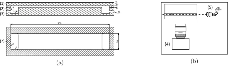
Figure 2: (a) Acrylic test piece containing rectangular channel 300 mmlong ×30 mm wide×
4.2 mm high, (1) cover plate, (2) channel plate, and (3) base plate with inlet and outlet, (b) Orientation of (4) camera and (5) laser light sheet optics to capture the velocity profile.
ν∇2U0−dU0
dt =
1
ρ∇P
0 (1)
where ρ and ν are the density and kinematic viscosity of the fluid, ∇2 = δ2/δy2 +δ2/δz2 is
the two-dimensional Laplacian operator, and∇P0 =dP0/dxis the oscillating pressure gradient. The origin is set at the lower left corner of the channel such that 0 ≤ y ≤ a and 0 ≤ z ≤ b. Equation 1 may be integrated over a cross-section to give the momentum balance equation:
Γ
A·¯τ 0
w+ρ dU¯0
dt =∇P
0 (2)
where Γ is the perimeter length, ¯τw0 is the perimeter mean of the wall shear stress and ¯U0 is the mean velocity. Equation 2 quantifies the pressure drop in a channel, resulting from viscous and inertial contributions. The linearity of Equations 1 and 2 allows the steady and time-dependent components to be decoupled. The Green function for velocity is [8]:
GU(y, z, t) =
16
π2
∞ X
m=0
∞ X
n=0
Z
(2m+ 1)(2n+ 1)·e
−νβt (3)
where:
Z =sin(2m+ 1)πy
a sin
(2n+ 1)πz
b ; β =
π2(2m+ 1)2
a2 +
π2(2n+ 1)2
b2 (4)
The solution for the local instantaneous time-dependent velocity is attained by convolving
GU with a sinusoidally oscillating accelerative functionf(t) = (1/ρ)∇Pt·cos(ωt):
U0(y, z, t) =−16∇Pt
ρπ2
∞ X
m=0
∞ X
n=0
Z
(2m+ 1)(2n+ 1)·
νβcos(ωt) +ωsin(ωt)−νβe−νβt
ν2β2+ω2 (5)
Solutions for flow rate Q0(t) and cross-sectional flow rate at the channel mid-height Q0cs(t) have been reported in a previous study [10]. ∇Pt is determined using the latter expression
with computed integrals of the phase-averaged experimental velocity profiles. Starting from rest, these quantities will contain transients for a period after the motion starts governed by the
[image:4.595.82.486.112.225.2]0 1 2 3 4 5 −1.5
−1
ω t [rad]
τw2/τw2,0
∇P′
/∇P0 Q′
/Q0
(a)
10−1 100 101 102
0
Wo
(b)
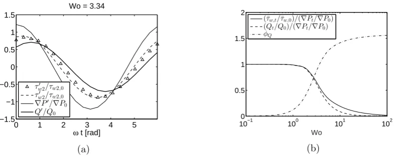
Figure 4: (a) Temporal evolution of τw02/τw2,0 at channel mid-height, ∇P0/∇P0 and Q0/Q0 for
W o= 3.33,Qt/Q0 = 0.7, (b) Evolution of amplitudes and phases of ¯τw0 /τ¯w,0andQ0/Q0withW o.
Lines and symbols represent analytical solutions and experimental measurements respectively.
τw02(z, t) =−16ν∇Pt
πa ∞ X
m=0
∞ X
n=0
sin[(2n+ 1)πz/b] (2n+ 1) ·
νβcos(ωt) +ωsin(ωt)−νβe−νβt
ν2β2+ω2 (6)
The mean value at each wall is ¯τw02 = (1/b)Rb
0 τw02dz. The mean over the entire perimeter ¯τw0
is the weighted mean of the individual wall averages ¯τw0 = (aτ¯w01+bτ¯w02)/(a+b).
3. Experimental 3.1. Apparatus
3.1.1. Channel Test Section The test piece consists of a single rectangular channel 300 mm
long ×30 mmwide× 4.2mmhigh laser cut from optically transparent acrylic, covered above and below by acrylic pieces. The inlet and outlet are machined into the base piece, as illustrated in Figure 2(a). Sealing is achieved using silicone rubber gaskets. The viewing window is 75mm
long, centered in the 300 mmlength to reduce asymmetrical effects. To facilitate optical access through the narrow edge of the channel plate, the machined surfaces are polished.
3.1.2. Gear Pump Pulsator The flow is driven by a micro annular gear pump (HNP
Mikrosysteme mzr-4605, 72 mL/min) and operated using a Terminal Box S-G05 controller and Matlab software. Pulsating flow of a given mean, frequency and amplitude is generated by discretising the corresponding sinusoid into a finite number of time steps. At each interval, a timer function executes and writes a motor speed to the controller based on the phase of the period. A maximum step size of 0.5 s is used to ensure that the inertia of the motor causes a smooth temporal flow rate. A counter implemented in the timer function records the phase of the output flow. At desired phase values, a digital output pin on the motor controller is set to high and sent to the imaging system to trigger image capture.
3.1.3. Particle Image Velocimetry The imaging system uses particle image velocimetry (PIV) to measure the local flow velocities. Collimated green (532 nm) light from a pair of Nd:YAG lasers (15Hz, 200mJ per pulse) is focused and diverged using concave and convex lenses (with focal lengths of 1000 mm and -25 mm respectively) to produce a laser plane of about 1 mm
thickness. The sheet illuminates the 4 µm diameter nylon-12 tracer particles (TSI P/N 10084)
[image:5.595.101.494.112.270.2]with which the fluid is seeded. Images of the flow are captured by a TSI 4 M P (2352 x 1768 pixels) PowerView CCD camera with a close-up Sigma DG 105 mm focal length macro lens, interfaced to the PC using an Xcelera frame grabber. The camera and laser system are aligned at right angles to each other to capture the velocity distribution across the 30 mm channel width, as illustrated in Figure 2(b). System timing is controlled by a Model 610035 LaserPulse Synchroniser. This control unit also reads an external 800µs TTL pulse trigger signal from the pump controller to phase-lock measurements to the sinusoidal oscillation of the flow. The entire PIV system is completely controlled by a dedicated computer running TSI’s Insight 4G data acquisition software.
0 π 2π 3π
−1 −0.5 0 0.5
1 Wo = 1.49
ωt [rad]
∇P′
/∇Pt
ρ(dU¯′/dt)/∇Pt
(Γ/A)¯τ′
w/∇Pt
(Q′
/Q0)/(∇Pt/∇P0)
0 π 2π 3π
−1 −0.5 0 0.5
1 Wo = 3.33
ωt [rad]
0 π 2π 3π
−1 −0.5 0 0.5
1 Wo = 10.54
ωt [rad] 0 π 2π 3π
−1 −0.5 0 0.5
1 Wo = 33.33
[image:6.595.134.525.248.394.2]ωt [rad]
Figure 5: Instantaneous viscous and inertial contributions to the overall pressure gradient for
W o= 1.49, 3.33, 10.54 and 33.33.
4. Results & Discussion
In this section, the experimental and theoretical results for pulsating flows with Reynolds numbers Re0 = 34, W o = 1.49, 3.33 and 10.54 (f = 0.02, 0.1 and 1 Hz) are presented. For
completeness, pulsations with a very high Womersley numberW o= 33.33 (f = 10 Hz), which is unachievable with the gear pump pulsator, are studied analytically. The absence of inertia (dU¯0/dt = 0) in the steady components of these flows results in a mean pressure drop that is entirely as a result of shear stress at the walls of the channel. Thus, only the oscillating components of the flow are considered, which are computed through subtraction of the mean steady profile solution Re0 = 34 from the pulsating profiles.
4.1. Wall shear stress and pressure gradient
To determine the wall shear stress at the midpoint of the channel height τw02(b/2, t), the slope between the vector nearest the wall (y = 0.3 mm) and the wall itself is computed from the velocity data. Plotted by the symbols of Figure 4(a) for the example case of W o= 3.33, these experimental values are in good agreement with that predicted by theory. The pressure gradient and the wall shear stress lead the flow rate by 0.63 and 0.31 radians, respectively. Withτw01(y, t) and all but one point on τw02(z, t) unknown, estimation of the overall mean wall shear stress is difficult and analysis is confined to theory.
Figure 4(b) plots the amplitudes and phases of the space-averaged wall shear stress ¯τw,t/τ¯w,0
and the flow rate Qt/Q0, normalised by the pressure gradient ∇Pt/∇P0, as a function of
frequencies. A phase lag develops at higher frequencies that tends to π/2 radians.
10−1 100 101 102
0 0.2 0.4 0.6 0.8 1
Wo
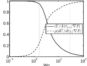
[image:7.595.223.368.239.348.2](Γ/A)¯τw,t/∇Pt ρ(dU /dt¯ )t/∇Pt
Figure 6: Viscous and inertial stress oscillation amplitudes, normalised by the pressure gradient amplitude, as a function of frequency. Vertical lines delineate the frequency regime boundaries.
4.2. Viscous and inertial stresses
The relationship between the viscous (Γ/A)¯τw0, inertial ρdU¯0/dt, and pressure gradient ∇P0
terms may be investigated through the momentum integral equation (Equation 2). Figure 5 illustrates that the relative contributions of the individual stresses to the overall pressure drop varies with time for a given frequency, based on the phases and amplitudes of the individual terms. Also plotted are the temporal evolutions of the flow rate oscillations (Q0/Q0)/(∇Pt/∇P0),
which always lag the inertial terms by π/2 radians. The amplitudes of these terms capture the increase in magnitudes of pressure oscillations relative to the flow rate oscillations. For the slowest oscillations, the acceleration of the fluid is negligible and viscous losses dominate. The flow is quasi-steady with the overall pressure gradient oscillating in phase with the viscous stress at the wall of the channel. Further, the flow rate has the same amplitude as and oscillates in phase with the pressure gradient. As the frequency is increased to W o = 3.33, the value of the inertia term becomes appreciable, with an amplitude similar to that of the viscous term. Thus, the flow is in the transitional regime and the resultant phase of the pressure gradient is somewhere between that of the individual contributions. A phase difference appears between the pressure gradient and the flow rate, and (Q0/Q0)/(∇Pt/∇P0) decreases due to the augmented
oscillating pressure gradient. At W o = 10.54, the majority (though less than 95%) of losses in the system are caused by inertia and the pressure gradient phase approaches that of the inertial term. Moreover, the phase delay between the driving pressure difference and the flow rate increases and∇Ptincreases further compared toQ0. ForW o= 33.33, the pressure drop in
the channel is mostly due to and varies in phase with the acceleration of the fluid. The flow is in the inertia-dominated regime with the pressure gradient leading the rate of flow byπ/2 radians.
4.3. Critical points of transition
Ohmi et al. [12] defined boundaries to the various regimes based on adherence to a certain mathematical approximation. With few inertial losses in the system, the flow is quasi-steady. When the majority of the pressure drop is due to inertia, the assumption of inviscid flow
holds. This definition is hence useful for reducing the calculation times of hydrodynamic models in engineering applications. In Figure 6, which plots the amplitudes of viscous and inertial forces relative to that of the pressure gradient as a function of oscillation speed, three unique frequency regimes may be distinguished: the region where the amplitude of the viscous term is approximately the same as that of the pressure gradient, the region where the amplitude of the inertial stress is close to that of the pressure gradient, and the range of frequencies between where the amplitude of both contributing terms are significant. Using 5% limits, the critical frequencies are found to be W o= 1.6 and 28.4, compared to W o= 1.32 and 28 for pipe flow. Incidentally, it should be noted that the amplitudes of the stress contributors, ρ(dU¯0/dt)/∇Pt
and (Γ/A)¯τw0/∇Pt, do not necessarily sum to one, as is well illustrated in Figure 5 for W o =
3.33.
0 5 10 15
−4 −3 −2 −1 0 1 2 3 4 y8[mm] U8[mm/s] (b)8Wo8=83.33 Analytic π/10 3π/10 5π/10 7π/10 9π/10 11π/10 13π/10 15π/10 17π/10 19π/10
0 5 10 15
−4 −3 −2 −1 0 1 2 3 4 y8[mm] U8[mm/s] (a)8Wo8=81.49 Analytic π/10 3π/10 5π/10 7π/10 9π/10 11π/10 13π/10 15π/10 17π/10 19π/10
0 5 10 15
−4 −3 −2 −1 0 1 2 3 4 y8[mm] U8[mm/s] (c)8Wo8=810.54 Analytic 0 2π/10 4π/10 6π/10 8π/10 10π/10 12π/10 14π/10 16π/10 18π/10
0 5 10 15
[image:8.595.74.525.268.401.2]−4 −3 −2 −1 0 1 2 3 4 y8[mm] U8[mm/s] (d)8Wo8=833.33 Analytic π/10 3π/10 5π/10 7π/10 9π/10 11π/10 13π/10 15π/10 17π/10 19π/10 19π/10
Figure 7: Phase-averaged oscillating velocity profiles for (a) W o = 1.49 (f = 0.02 Hz) and
Qt/Q0 = 0.7, (b) W o= 3.33 (f = 0.1Hz) andQt/Q0 = 0.7, (c) W o= 10.54 (f = 1 Hz) and
Qt/Q0= 1, and (d)W o= 33.33 (f = 10Hz) andQt/Q0 = 1. Solid lines and symbols represent
analytical solutions and experimental measurements respectively.
4.4. Velocity Profiles
The evolving relationship between viscous and inertial stresses with frequency results in distinct velocity distributions dependent on the regime of unsteadiness. The unique characteristics predicted, which are apparent in both the experimental and theoretical profiles of Figure 7, owe primarily to the growing phase delays in the system. The quasi-steady profile closely resembles that of steady flow (with some unsteady effects still observable) and local velocity oscillations are universally in phase. With increasing frequency, a lag appears between the main fluid body and the accelerating pressure gradient as discussed in Section 4.1. Near the wall however, viscous stresses reduce the momentum of fluid layers, which are inclined to reverse quickly when the pressure gradient reverses, leading to the observed annular effects of the mid-frequency velocity profiles. The overshoot continues to grow and move closer to the wall. This leads to what is essentially plug flow, as seen in the theoretical inertia-dominated velocity profile.
parameters were found to augment, with the latter growing at a faster rate than the former. Inertial losses were identified as the cause of the high pressure drops, whose overall contribution was also investigated with frequency. Since each flow exhibits unique characteristics that may affect heat transfer, boundaries to the quasi-steady, transitional and inertia-dominated regimes were defined in a rectangular channel using the definition of Ohmi et al. [12], which is based on the adherence of the flow to mechanical models.
In practical applications, it is possible that a trade-off exists where heat transfer enhancement is balanced by increased pressure demands. While the high shear rates of the inertia-dominated regime are desirable, the very large pressure drops are probably unfeasible, especially in microchannels where high frequencies to the order of kHz are required. The ratio of the wall shear stress to the pressure drop augmentation acts as a performance indicator using solely fluid mechanical parameters.
Acknowledgments
The authors would like to acknowledge the financial support of the Irish Research Council (IRC) under grant number EPSPG/2013/618.
References
[1] T. Persoons, T. Saenen, T. Van Oevelen, and M. Baelmans, “Effect of flow pulsation on the heat transfer performance of a minichannel heat sink,”Journal of Heat Transfer, vol. 134, no. 9, p. 091702, 2012. [2] N. Jeffers, J. Stafford, K. Nolan, B. Donnelly, R. Enright, J. Punch, A. Waddell, L. Erlich, J. O’Connor,
A. Sexton, R. Blythman, and D. Hernon, “Microfluidic cooling of photonic integrated circuits (PICs),” in
Fourth European Conference on Microfluidics, Limerick, Ireland, 2014.
[3] G. Stokes, On the effect of the internal friction of fluids on the motion of pendulums, vol. 9. Pitt Press, 1851.
[4] J. Womersley, “Method for the calculation of velocity, rate of flow and viscous drag in arteries when the pressure gradient is known,”The Journal of Physiology, vol. 127, no. 3, pp. 553–563, 1955.
[5] T. Sexl, “ ¨Uber den von E.G. Richardson entdeckten annulareffekt ,”Zeitschrift f¨ur Physik, vol. 61, no. 5-6, pp. 349–362, 1930.
[6] S. Uchida, “The pulsating viscous flow superposed on the steady laminar motion of incompressible fluid in a circular pipe,”Zeitschrift f¨ur angewandte Mathematik und Physik ZAMP, vol. 7, no. 5, pp. 403–422, 1956. [7] H. Ito, “Theory of laminar flow through a pipe with non-steady pressure gradients,” Proceedings of the
Institute of High Speed Mechanics, p. 163, 1953.
[8] C. Fan and B. Chao, “Unsteady, laminar, incompressible flow through rectangular ducts,” Zeitschrift f¨ur angewandte Mathematik und Physik ZAMP, vol. 16, no. 3, pp. 351–360, 1965.
[9] T. Zhao and P. Cheng, “The friction coefficient of a fully developed laminar reciprocating flow in a circular pipe,”International Journal of Heat and Fluid Flow, vol. 17, no. 2, pp. 167–172, 1996.
[10] R. Blythman, N. Jeffers, T. Persoons, and D. Murray, “Localized and time-resolved velocity measurements of pulsatile flow in a rectangular channel,” inEighteenth International Conference on Fluid Mechanics and Thermodynamics, Rio de Janeiro, Brazil, 2016.
[11] S. Ray, B. ¨Unsal, F. Durst, ¨O. Ertunc, and O. Bayoumi, “Mass flow rate controlled fully developed laminar pulsating pipe flows,”Journal of Fluids Engineering, vol. 127, no. 3, pp. 405–418, 2005.
[12] M. Ohmi, M. Iguchi, and T. Usui, “Flow pattern and frictional losses in pulsating pipe flow: Part 5, wall shear stress and flow pattern in a laminar flow,”Bulletin of JSME, vol. 24, no. 187, pp. 75–81, 1981. [13] K. Haddad, ¨O. Ertun¸c, M. Mishra, and A. Delgado, “Pulsating laminar fully developed channel and pipe
flows,”Physical Review E, vol. 81, no. 1, p. 016303, 2010.